ANOVA Test in Python
The following tutorial is based on data analysis; we will discuss the Analysis of Variance (ANOVA) in detail, along with the process of carrying it out in the Python programming language. ANOVAs are generally utilized in Psychology studies.
In the following tutorial, we will understand how we can carry out ANOVA with the help of the SciPy library, evaluating it “by hand” in Python, utilizing Pyyttbl and Statsmodels.
Understanding the ANOVA Test
We can think of an Analysis of Variance Test, also known as ANOVA, to generalize the T-tests for multiple groups. Generally, we use the independent T-test in order to compare the means of the state between two groups. We use ANOVA Test whenever we need a comparison of the means of the state between more than two groups.
ANOVA test checks whether a difference in the average somewhere in the model or not (checking whether there was an overall effect or not); however, this method doesn’t tell us the spot of the difference (if there is one). We can find the spot of the difference between the group by conducting the post hoc tests.
However, in order to perform any tests, we first have to define the null and alternate hypotheses:
- Null Hypothesis:There is no noteworthy difference between the groups.
- Alternate Hypothesis:There is a noteworthy difference between the groups.
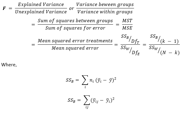
We can perform an ANOVA Test by comparing two types of variations. The First variation is between the sample means and the other one within each of the samples. The formula shown below describes one-way ANOVA Test statistics.
The output of the ANOVA formula, the F statistic (also known as the F-ratio), enables the analysis of the multiple sets of data in order to determine the variability among the samples and within samples.
We can write the formula for the One-way ANOVA test as illustrated below:
Where,
yi – Sample Mean in the ith group
ni – Number of Observation in the ith group
y – Total mean of the data
k – Total number of the groups
yij – jth observation in the out of k groups
N – Overall sample size
Whenever we plot the ANOVA table, we can see all the above components in the following format:
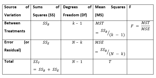
Usually, if the p-value belonging to the F is smaller than 0.05, then the null hypothesis is excluded, and the alternative hypothesis is maintained. In the case of the null hypothesis rejection, we can say that the means of all the sets/groups aren’t equal.
Note: If no real difference is present among the tested groups, which is known as the null hypothesis, the F-ratio statistics of the ANOVA Test will be adjacent to 1.
ANOVA Test Assumptions
Before performing an ANOVA test, we must make certain assumptions, as shown below:
- We can obtain observations randomly and independently from the population defined by the factor levels.
- The data for every level of the factor is distributed generally.
- Case Independent: The sample cases must be independent of each other.
- Variance Homogeneity: Homogeneity signifies that the variance between the group needs to be around equal.
We can test the assumption of variance homogeneity with the bits of help of tests like the Brown-Forsythe Test or Levene’s Test. We can also test the Normality of the score distributions with the help of histograms, the kurtosis or skewness values, or with the help of tests like Kolmogorov-Smirnov, Shapiro-Wilk, or Q-Q plot. We can also determine the assumption of independence from the study design.
It is quite noteworthy to notice that the ANOVA test is not robust to violating the assumption of independence. This is to inform that even if someone tries to violate the assumptions of Normality or homogeneity, they can conduct the test and trust the findings.
Nevertheless, the outputs of the ANOVA test are unacceptable if the assumption of independence is dishonored. Usually, the analysis, along with the violations of homogeneity, is considered robust if we have equal-sized groups. Resuming the ANOVA test along with violations of Normality is usually fine if we have a large sample size.
Understanding the Types of ANOVA Tests
The ANOVA Tests can be classified into three major types. These types are shown below:
- One-Way ANOVA Test
- Two-Way ANOVA Test
- n-Way ANOVA Test
One-Way ANOVA Test
An Analysis of Variance Test that has only one independent variable is known as the One-way ANOVA Test.
For instance, a country can assess the differences in the cases of Coronavirus, and a Country can have multiple categories for comparison.
Two-Way ANOVA Test
An Analysis of Variance Test that has two independent variables is known as a Two-way ANOVA test. This test is also known as Factorial ANOVA Test.
For example, expanding the above example, a two-way ANOVA can examine the difference in the cases of Coronavirus (the dependent variable) by Age Group (the first independent variable) and Gender (the second independent variable). The two-way ANOVA can be utilized in order to examine the interaction among these two independent variables. Interactions denote that the differences are uneven across all classes of the independent variables.
Suppose that the old age group may have higher cases of Coronavirus overall compared to the young age group; however, this difference could vary in countries in Europe compared to countries in Asia.
n-Way ANOVA Test
An Analysis of Variance Test is considered an n-way ANOVA Test if a researcher uses more than two independent variables. Here n represents the number of independent variables we have. This Test is also known as MANOVA Test.
For example, we can examine potential differences in cases of Coronavirus using independent variables like Country, Age group, Gender, Ethnicity, and a lot more simultaneously.
An ANOVA Test will provide us a single (univariate) F-value; however, a MANOVA Test will provide us a multivariate F-value.
Understanding with Replication and without Replication in ANOVA
Generally, some of us may hear with replication and without replication in respect to the ANOVA test. Let us understand what these are:
Two-way ANOVA test with Replication
The two-way ANOVA test with Replication is carried out when two groups and the members of those groups are performing multiple tasks.
For instance, suppose that a vaccine for Coronavirus is still under development. Doctors are performing two different treatments in order to cure two groups of patients infected by the virus.
Two-way ANOVA test without Replication
The two-way ANOVA test without Replication is carried out when we have only one group, and we are double-testing that same group.
For instance, suppose that the vaccine has been developed successfully, and the researchers are testing one set of volunteers before and after they have been vaccinated in order to observe whether the vaccination is working properly or not.
Understanding the Post-ANOVA Test
While conducting an ANOVA Test, we are trying to determine the statistically significant difference between the groups, if it is available. In case we find one, we will then have to test where the spot of group differences.
Thus, the researcher uses the post hoc test in order to check which groups are different from each other.
We could perform post hoc tests which are t-tests inspecting mean differences among the groups. We can conduct several multiple comparison tests to control the Type I error rate, including the Bonferroni, Dunnet, Scheffe, and Turkey tests.
Now, we will understand only one-way ANOVA test using the Python programming language.
Understanding One-way ANOVA test in Python
We have divided the process of performing the ANOVA test into different sections.
Importing required libraries
In order to begin working with the ANOVA test, let us import some necessary libraries and modules for the project.
Syntax:
The Hypothesis
Let us consider a hypothesis for the problem:
“For every diet, the mean of the people’s weights is the same.”
Loading the Data
In the following problem, we will use a Diet dataset designed by the University of Sheffield. The dataset contains a binary variable as the gender, which consists of 1 for Male and 0 for Female.
Let us consider the following syntax for the same:
Syntax:
Understanding the Dataset
Once we have successfully imported the dataset, let us print some data to get a sense of it.
Example –
Output:
Person gender Age Height pre.weight Diet weight6weeks 0 25 41 171 60 2 60.0 1 26 32 174 103 2 103.0 2 1 0 22 159 58 1 54.2 3 2 0 46 192 60 1 54.0 4 3 0 55 170 64 1 63.3
Now let us print the total number of rows present in the dataset.
Example –
Output:
The total number of rows in the dataset: 546
Checking the Missing Values
Now, we have to see if there are any values that are missing in the dataset or not. We can check this by using the following syntax.
Example –
Output:
[' ' '0' '1'] Person gender Age Height pre.weight Diet weight6weeks 0 25 41 171 60 2 60.0 1 26 32 174 103 2 103.0
We can observe that two entries are containing the missing values in the ‘gender’ column. Now let us find the total percentage of missing values in the dataset.
Example –
Output:
Percentage of missing values in the dataset: 2.56%
As we can observe, we have approximately 3% of missing values in the dataset. We can either ignore, delete, or classify its gender with the help of the closest Height mean.
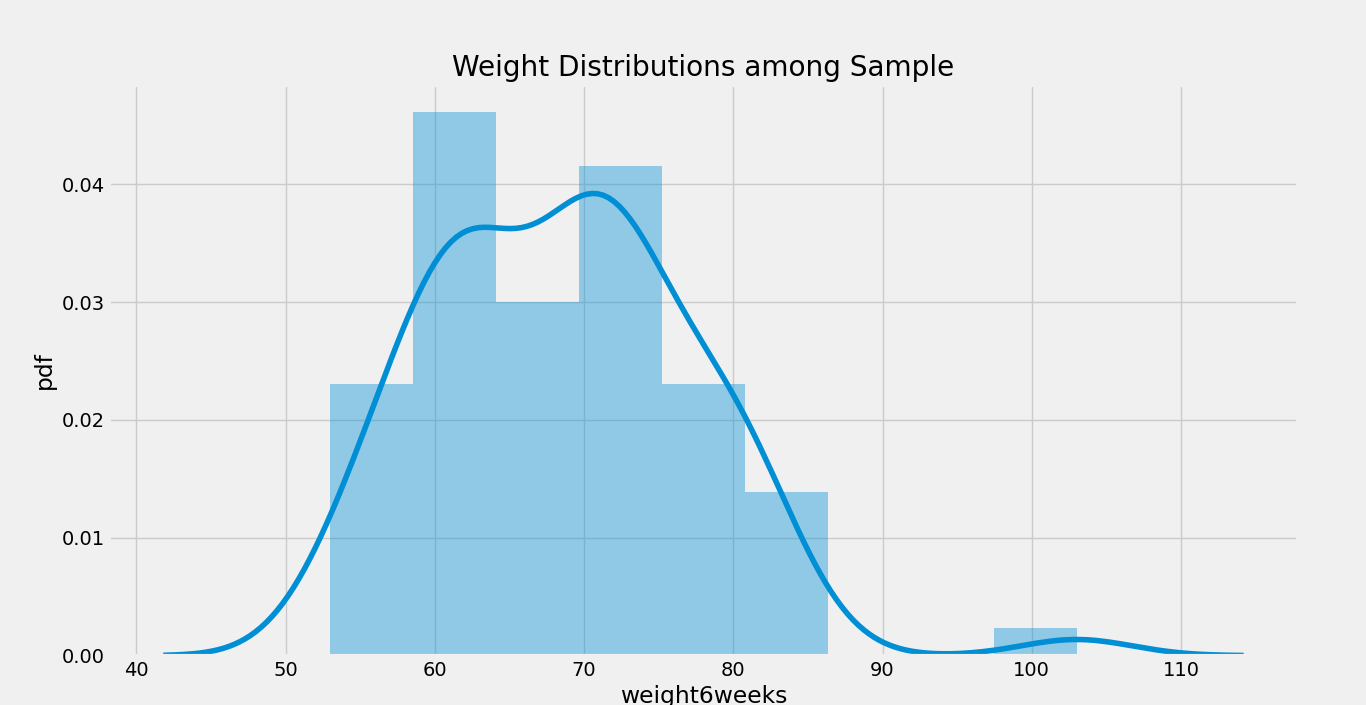
Understanding the distribution of Weight
In the following step, we will be plot a graph using the distplot() function to understand the Weight distribution in the Sample data. Let us consider the snippet of code.
Example –
Output:
We can also plot a distribution plot for each Gender in the dataset. Here is a syntax for the same:
Example –
Output:
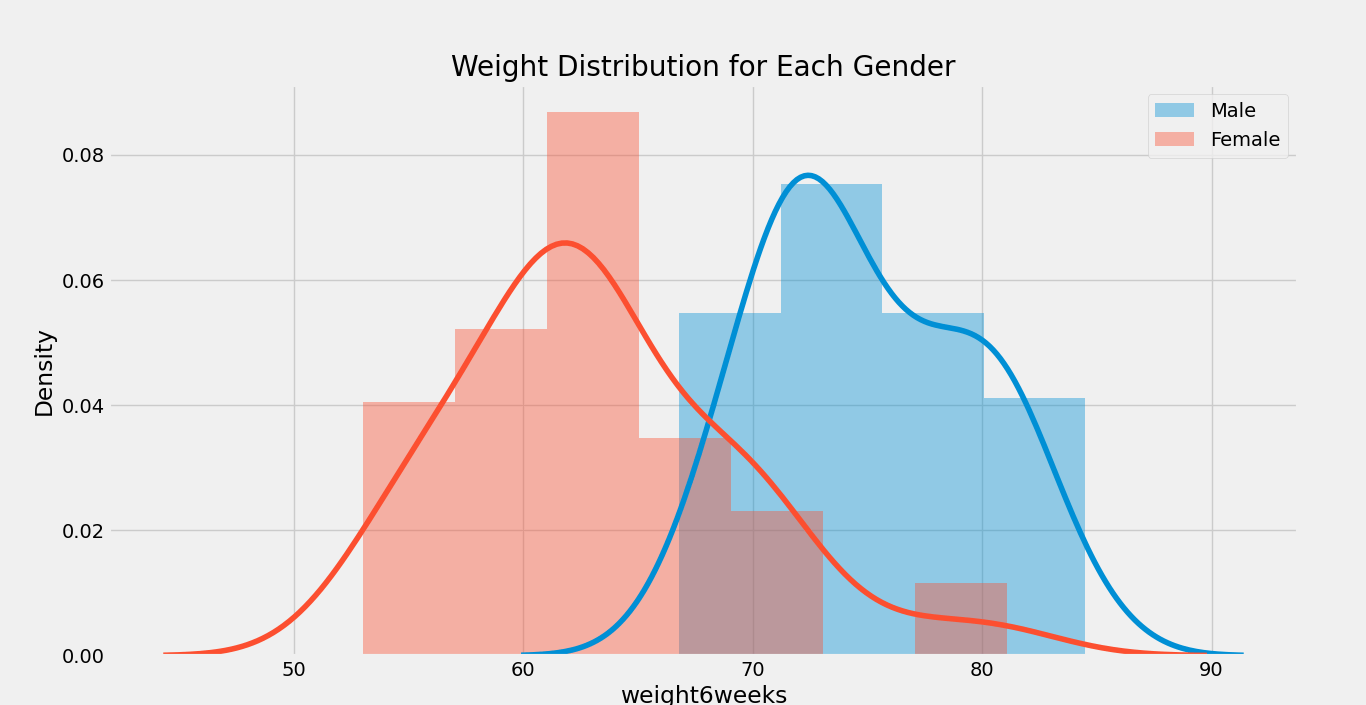
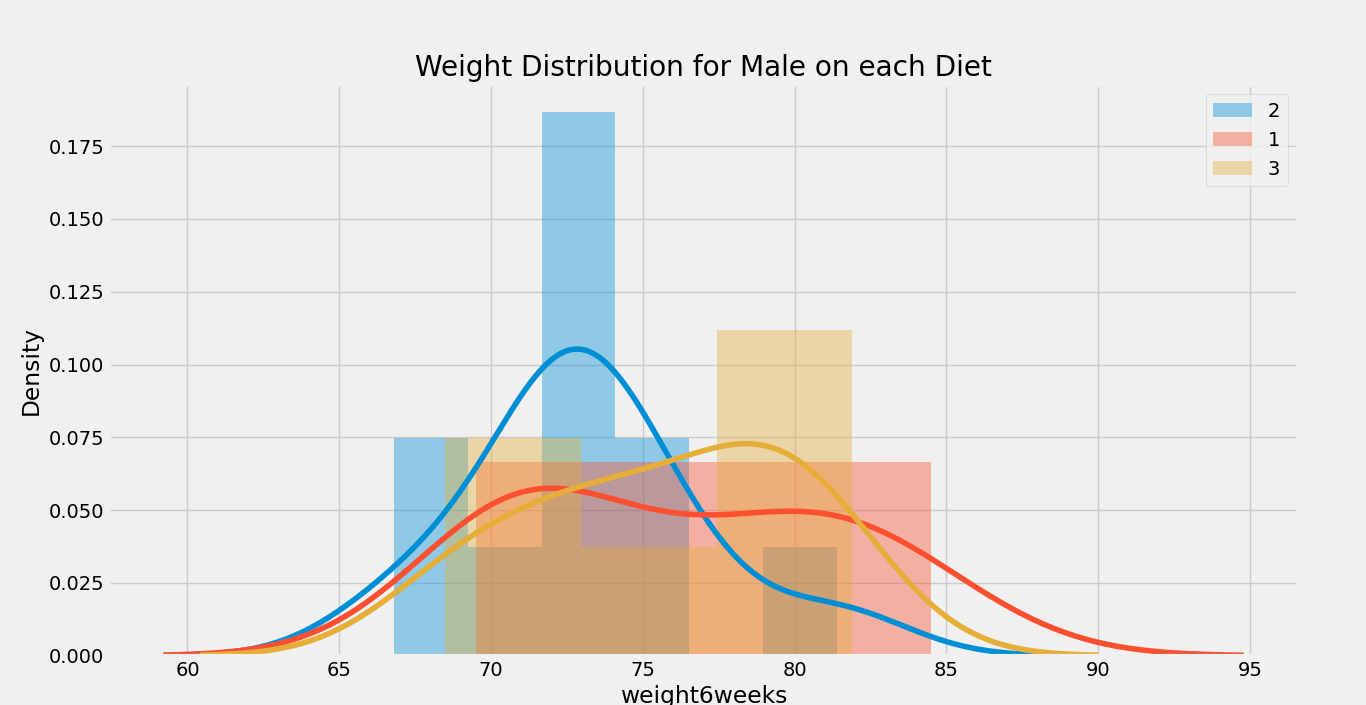
We can also use the following function to display the distribution plot for each gender.
Example:
Output:
Graph 1:
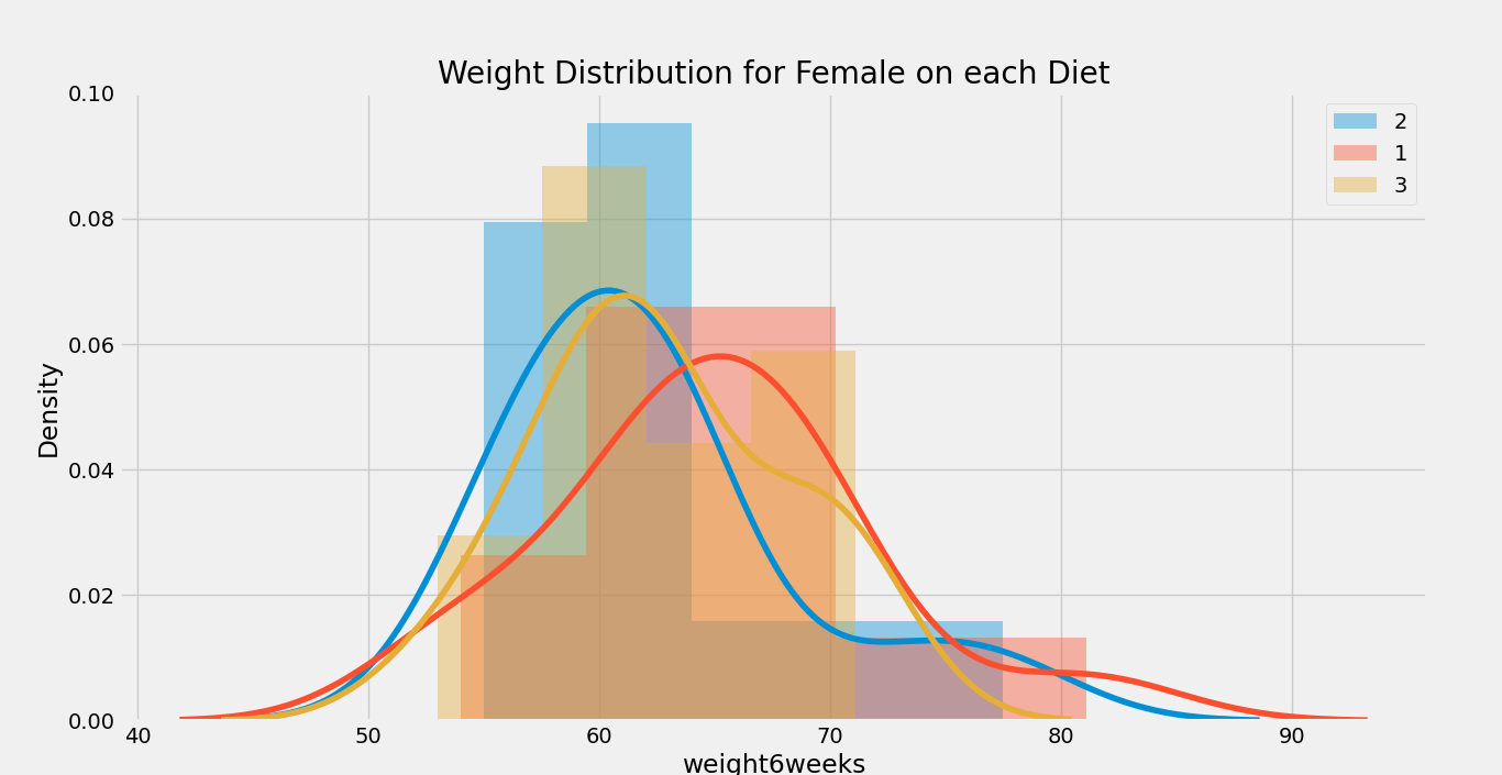
Graph 2:
Now, we will calculate the mean, median, non-zero count, and standard deviation according to the ‘gender’ column using the snippet of code given below:
Example –
Output:
mean median count_nonzero std gender 81.500000 81.5 2.0 30.405592 0 63.223256 62.4 43.0 6.150874 1 75.015152 73.9 33.0 4.629398
As we can observe, we have estimated the required statistical measurements on the basis of gender. We can also classify these statistical measurements on the basis of gender as well as diet.
Example –
Output:
mean median count_nonzero std gender Diet 2 81.500000 81.50 2.0 30.405592 0 1 64.878571 64.50 14.0 6.877296 2 62.178571 61.15 14.0 6.274635 3 62.653333 61.80 15.0 5.370537 1 1 76.150000 75.75 10.0 5.439414 2 73.163636 72.70 11.0 3.818448 3 75.766667 76.35 12.0 4.434848
We can observe that there is a slight difference in weight on females in the diet; however, it doesn’t seem to affect males.
Performing the one-way ANOVA Test
The null hypothesis of the one-way ANOVA test is
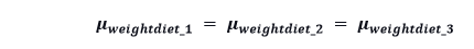
And this test attempts to check whether this hypothesis is true or not.
Let us consider initially determining the confidence level of 95%, which also implies that we will accept only an error rate of 5%.
Example –
Output:
ANOVA table for Female ---------------------- sum_sq df F PR(>F) Diet 559.680764 1.0 7.17969 0.010566 Residual 3196.086677 41.0 NaN NaN ANOVA table for Male ---------------------- sum_sq df F PR(>F) Diet 559.680764 1.0 7.17969 0.010566 Residual 3196.086677 41.0 NaN NaN
In the above output, we can observe two p-values (PR (> F)): male and female.
In the case of males, we can’t accept the null hypothesis below the confidence level of 95% because the p-value is larger than the value of alpha, i.e., 0.05 < 0.512784. Thus, no difference is found in the weights of males after providing these three types of diet.
In the case of females, since the p-value PR (> F) is below the rate of error, i.e., 0.05 > 0.010566, we could reject the null hypothesis. This statement indicates that we are pretty confident about the fact that there is a difference in terms of height for females in diets.
So, now we understand the effect of diet on females; however, we are not aware of the difference between the diets. So, we will perform a post hoc analysis with the help of the Tukey HSD (Honest Significant Difference) test.
Let us consider the following snippet of code for the same.
Example –
Output:
Multiple Comparison of Means - Tukey HSD, FWER=0.05 ===================================================== group1 group2 meandiff p-adj lower upper reject ----------------------------------------------------- 1 2 -3.5714 0.5437 -11.7861 4.6432 False 1 3 -8.7714 0.0307 -16.848 -0.6948 True 2 3 -5.2 0.2719 -13.2766 2.8766 False ----------------------------------------------------- Unique diet groups: [1 2 3]
As we can observe from the above output, we can only reject the null hypothesis among the 1st and 3rd types of diet, which means that a statistically significant difference is present in weight for diet 1 and diet 3.