73

Back Propagation through time – RNN

Introduction:

Recurrent Neural Networks are those networks that deal with sequential data. They can predict outputs based on not only current inputs but also considering the inputs that were generated prior to it. The output of the present depends on the output of the present and the memory element (which includes the previous inputs).

To train these networks, we make use of traditional backpropagation with an added twist. We don’t train the system on the exact time “t”. We train it according to a particular time “t” as well as everything that has occurred prior to time “t” like the following: t-1, t-2, t-3.

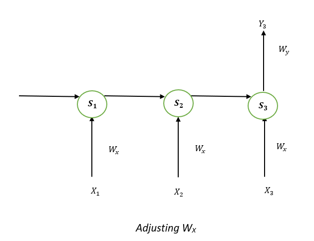
Take a look at the following illustration of the RNN:

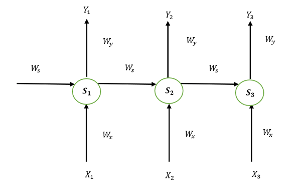
S1, S2, and S3 are the states that are hidden or memory units at the time of t1, t2, and t3, respectively, while Ws represents the matrix of weight that goes with it.

X1, X2, and X3 are the inputs for the time that is t1, t2, and t3, respectively, while Wx represents the weighted matrix that goes with it.

The numbers Y1, Y2, and Y3 are the outputs of t1, t2, and t3, respectively as well as Wy, the weighted matrix that goes with it.

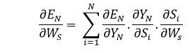
For any time, t, we have the following two equations:

S_t = g₁ (W_x x_t + W_s S_t-1)
Y_t = g₂ (W_Y S_t )

where g1 and g2 are activation functions.

We will now perform the back propagation at time t = 3.

Let the error function be:

E_t=(d_t-Y_t )²

Here, we employ the squared error, in which D3 is the desired output at a time t = 3.

In order to do backpropagation, it is necessary to change the weights that are associated with inputs, memory units, and outputs.

Adjusting W_y

To better understand, we can look at the following image:

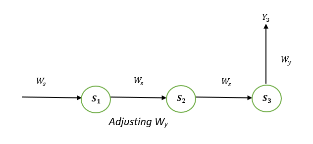
Explanation:

E₃ is a function of Y₃. Hence, we differentiate E₃ with respect to Y₃.

Y₃ is a function of W₃. Hence, we differentiate Y₃ with respect to W₃.

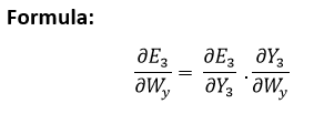
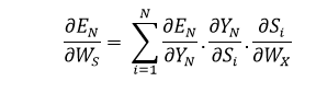
Adjusting Ws

To better understand, we can look at the following image:

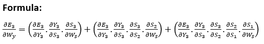
Explanation:

E₃ is a function of the Y₃. Therefore, we distinguish the E₃ with respect to Y₃. Y₃ is a function of the S₃. Therefore, we differentiate between Y₃ with respect to S₃.

S₃ is an element in the W_s. Therefore, we distinguish between S₃ with respect to W_s.

But it’s not enough to stop at this, therefore we have to think about the previous steps in time. We must also differentiate (partially) the error function in relation to the memory units S₂ and S₁, considering the weight matrix W_s.

It is essential to be aware that a memory unit, such as S_t, is the result of its predecessor memory unit, S_t-1.

Therefore, we distinguish S₃ from S₂ and S₂ from S₁.

In general, we can describe this formula in terms of:

Adjusting W_X:

To better understand, we can look at the following image:

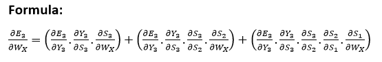
Explanation:

E₃ is an effect in the Y₃. Therefore, we distinguish the E₃ with respect to Y₃. Y₃ is an outcome that is a function of the S₃. Therefore, we distinguish the Y₃ with respect to S₃.

S₃ is an element in the W_X. Thus, we can distinguish the S₃ with respect to W_X.

We can’t just stop at this, and therefore we also need to think about the preceding time steps. Therefore, we separate (partially) the error function in relation to the memory unit S₂ and S₁, considering the W_X weighting matrix.

In general, we can define this formula in terms of:

Limitations:

This technique that uses the back Propagation over time (BPTT) is a method that can be employed for a limited amount of time intervals, like 8 or 10. If we continue to backpropagate and the gradient gets too small. This is known as the “Vanishing gradient” problem. This is because the value of information diminishes geometrically with time. Therefore, if the number of time steps is greater than 10 (Let’s say), the data is effectively discarded.

Going Beyond RNNs:

One of the most famous solutions to this issue is using what’s known as Long-Short-Term Memory (LSTM for short) cells instead of conventional RNN cells. However, there could be another issue, referred to as the explosion gradient problem, in which the gradient becomes uncontrollably high.

Solution:

A well-known method is known as gradient clipping when for each time step, we will determine if the gradient δ is greater than the threshold. If it is, then we should normalize it.

---