Basic concepts of root locus
In the previous sections, we have studies that the stability of a system. It depends on the location of the roots of the characteristic equation. We can also say that the stability of the system depends on the location of closed-loop poles. Such knowledge of the movement of the poles in the s-plane when the parameters are varied is important. The minor changes in the parameters can greatly help in the system designing. The nature of the system’s transient response is closely related to the location of the poles in the s-plane.
We have also studied the Routh Hurwitz criteria that describe the stability of the algebraic equation. If any of the term in the first column of the Roth table possesses a sign change, the system tends to become unstable.
The root locus method was introduced by W.R Evans in 1948. Root locus is a graphical method in which the movement of poles in the s-plane can be located when a specific parameter is varied from 0 to infinity. The parameter assumed to be varied is generally the gain of the system.
Consider the below closed loop system.
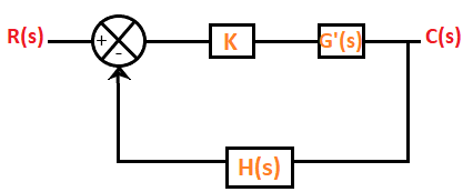
The equation of a closed loop system is given by:
1 + G(s)H(s) = 0
Where,
G(s) is the gain of the transfer function
H(s) is the feedback gain
In the case of root locus, the gain K is also assumed as part of the closed-loop system. K is known as system gain or the gain in the forward path. The characteristic equation after including the forward gain can be represented as:
1 + KG'(s)H(s) = 0
Where,
G(s) = KG'(s)
When the system includes the variable parameter K, the roots of the closed loop system are now dependent on the values of ‘K.’
The value of ‘K’ variable can vary in two cases, as shown below:
In the first case, for every different value (integer or decimal) of K, we will get separate set of locations of the roots. If all such locations are joined, the resulting plot is defined as the root locus. We can also define root locus as the locus of the closed loop poles obtained when the system gain ‘K’ is varied from -infinity to infinity.
When the K varies from zero to infinity, the plot is called the direct root locus. If the system gain ‘K’ varies from -infinity to zero, the plot thus obtained is known as inverse root locus. The gain K is generally assumed from zero to infinity unless specially stated.
Let’s consider an example.
Example: Obtain the root locus of the unity feedback system with G(s) = K/s.
As given, it is a unity feedback system. It means that H(s) = 1.
We know,
1 + G(s)H(s) = 0
1 + K/s = 0
S + K = 0
The roots of the above equation are located at s = -K.
As per the condition, the system gain K varies from zero to infinity unless states. Thus, we will obtain the root locus by joining all such locations when K varies from zero to infinity.
The values of the roots of the given equation at different values of K are given in the below table:
| K | S = -K Root Location |
| 0 | 0 |
| 1 | -1 |
| 5 | -5 |
| infinity | -infinity |
The plot of the root locus for the above values of K is shown below:
Uses of Root Locus
In addition in determining the stability of the system, root locus also helps to determine:
- Damping ratio
The damping ratio is a dimensionless unit that describes how the system decay affects the oscillations of the system. - Natural frequency
It is represented by wn. The value of the system gain K at the location of poles helps in computing the natural frequency and the damping ratio of the system. - P, PI, and PID controllers
P (proportional), PI (Proportional Integral), and PID (Proportional Integral Derivative) controllers can be designed with the help of root locus technique. Here, the input of the system to be controlled is made proportional to the system gain K. - Lag and lead compensators
The compensators are the additional components in the system added to compensate for deficient performance. The phase lead compensator helps to shift the root locus towards the left in the complex s-plane, and it further increases the system’s stability. Similarly, lag and lead compensators can be designed in various ways with the help of the root locus.
Advantages of Root locus
The advantages of root locus are as follows:
- We can analyze the absolute stability of the system with the help of a root locus plot.
- Using the magnitude and angle conditions, we can find the limiting value of the system gain K for any point on the root locus.
- Enhances system designing with better accuracy.
- It helps in analyzing the stability of the system with time delay.
- Root locus plots help us determine the gain margin, relative stability, phase margin, and the system’s settling time.
- The root locus technique is easy to implement as compared to other techniques in the control system.
- It helps in analyzing the performance of the control system.