73

BIRCH in Data Mining

BIRCH (balanced iterative reducing and clustering using hierarchies) is an unsupervised data mining algorithm that performs hierarchical clustering over large data sets. With modifications, it can also be used to accelerate k-means clustering and Gaussian mixture modeling with the expectation-maximization algorithm. An advantage of BIRCH is its ability to incrementally and dynamically cluster incoming, multi-dimensional metric data points to produce the best quality clustering for a given set of resources (memory and time constraints). In most cases, BIRCH only requires a single scan of the database.

Its inventors claim BIRCH to be the “first clustering algorithm proposed in the database area to handle ‘noise’ (data points that are not part of the underlying pattern) effectively”, beating DBSCAN by two months. The BIRCH algorithm received the SIGMOD 10 year test of time award in 2006.

Basic clustering algorithms like K means and agglomerative clustering are the most commonly used clustering algorithms. But when performing clustering on very large datasets, BIRCH and DBSCAN are the advanced clustering algorithms useful for performing precise clustering on large datasets. Moreover, BIRCH is very useful because of its easy implementation. BIRCH is a clustering algorithm that clusters the dataset first in small summaries, then after small summaries get clustered. It does not directly cluster the dataset. That is why BIRCH is often used with other clustering algorithms; after making the summary, the summary can also be clustered by other clustering algorithms.

It is provided as an alternative to MinibatchKMeans. It converts data to a tree data structure with the centroids being read off the leaf. And these centroids can be the final cluster centroid or the input for other cluster algorithms like Agglomerative Clustering.

Problem with Previous Clustering Algorithm

Previous clustering algorithms performed less effectively over very large databases and did not adequately consider the case wherein a dataset was too large to fit in main memory. Furthermore, most of BIRCH’s predecessors inspect all data points (or all currently existing clusters) equally for each clustering decision. They do not perform heuristic weighting based on the distance between these data points. As a result, there was a lot of overhead maintaining high clustering quality while minimizing the cost of additional IO (input/output) operations.

Stages of BIRCH

BIRCH is often used to complement other clustering algorithms by creating a summary of the dataset that the other clustering algorithm can now use. However, BIRCH has one major drawback it can only process metric attributes. A metric attribute is an attribute whose values can be represented in Euclidean space, i.e., no categorical attributes should be present. The BIRCH clustering algorithm consists of two stages:

1. Building the CF Tree: BIRCH summarizes large datasets into smaller, dense regions called Clustering Feature (CF) entries. Formally, a Clustering Feature entry is defined as an ordered triple (N, LS, SS) where ‘N’ is the number of data points in the cluster, ‘LS’ is the linear sum of the data points, and ‘SS’ is the squared sum of the data points in the cluster. A CF entry can be composed of other CF entries. Optionally, we can condense this initial CF tree into a smaller CF.
2. Global Clustering: Applies an existing clustering algorithm on the leaves of the CF tree. A CF tree is a tree where each leaf node contains a sub-cluster. Every entry in a CF tree contains a pointer to a child node, and a CF entry made up of the sum of CF entries in the child nodes. Optionally, we can refine these clusters.

Due to this two-step process, BIRCH is also called Two-Step Clustering.

Algorithm

The tree structure of the given data is built by the BIRCH algorithm called the Clustering feature tree (CF tree). This algorithm is based on the CF (clustering features) tree. In addition, this algorithm uses a tree-structured summary to create clusters.

In context to the CF tree, the algorithm compresses the data into the sets of CF nodes. Those nodes that have several sub-clusters can be called CF subclusters. These CF subclusters are situated in no-terminal CF nodes.

The CF tree is a height-balanced tree that gathers and manages clustering features and holds necessary information of given data for further hierarchical clustering. This prevents the need to work with whole data given as input. The tree cluster of data points as CF is represented by three numbers (N, LS, SS).

• N = number of items in subclusters
• LS = vector sum of the data points
• SS = sum of the squared data points

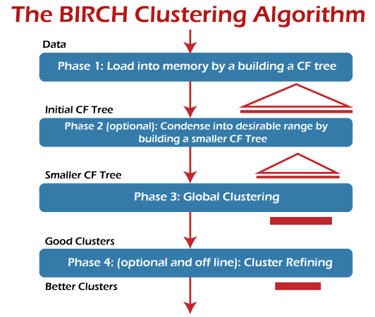
There are mainly four phases which are followed by the algorithm of BIRCH.

• Scanning data into memory.
• Condense data (resize data).
• Global clustering.
• Refining clusters.

Two of them (resize data and refining clusters) are optional in these four phases. They come in the process when more clarity is required. But scanning data is just like loading data into a model. After loading the data, the algorithm scans the whole data and fits them into the CF trees.

In condensing, it resets and resizes the data for better fitting into the CF tree. In global clustering, it sends CF trees for clustering using existing clustering algorithms. Finally, refining fixes the problem of CF trees where the same valued points are assigned to different leaf nodes.

Cluster Features

BIRCH clustering achieves its high efficiency by clever use of a small set of summary statistics to represent a larger set of data points. These summary statistics constitute a CF and represent a sufficient substitute for the actual data for clustering purposes.

A CF is a set of three summary statistics representing a set of data points in a single cluster. These statistics are as follows:

• Count [The number of data values in the cluster]
• Linear Sum [The sum of the individual coordinates. This is a measure of the location of the cluster]
• Squared Sum [The sum of the squared coordinates. This is a measure of the spread of the cluster]

NOTE: The linear sum and the squared sum are equivalent to the mean and variance of the data point.

CF Tree

The building process of the CF Tree can be summarized in the following steps, such as:

Step 1: For each given record, BIRCH compares the location of that record with the location of each CF in the root node, using either the linear sum or the mean of the CF. BIRCH passes the incoming record to the root node CF closest to the incoming record.

Step 2: The record then descends down to the non-leaf child nodes of the root node CF selected in step 1. BIRCH compares the location of the record with the location of each non-leaf CF. BIRCH passes the incoming record to the non-leaf node CF closest to the incoming record.

Step 3: The record then descends down to the leaf child nodes of the non-leaf node CF selected in step 2. BIRCH compares the location of the record with the location of each leaf. BIRCH tentatively passes the incoming record to the leaf closest to the incoming record.

Step 4: Perform one of the below points (i) or (ii):

1. If the radius of the chosen leaf, including the new record, does not exceed the threshold T, then the incoming record is assigned to that leaf. The leaf and its parent CF’s are updated to account for the new data point.
2. If the radius of the chosen leaf, including the new record, exceeds the Threshold T, then a new leaf is formed, consisting of the incoming record only. The parent CFs is updated to account for the new data point.

If step 4(ii) is executed, and the maximum L leaves are already in the leaf node, the leaf node is split into two leaf nodes. If the parent node is full, split the parent node, and so on. The most distant leaf node CFs are used as leaf node seeds, with the remaining CFs being assigned to whichever leaf node is closer. Note that the radius of a cluster may be calculated even without knowing the data points, as long as we have the count n, the linear sum LS, and the squared sum SS. This allows BIRCH to evaluate whether a given data point belongs to a particular sub-cluster without scanning the original data set.

Clustering the Sub-Clusters

Once the CF tree is built, any existing clustering algorithm may be applied to the sub-clusters (the CF leaf nodes) to combine these sub-clusters into clusters. The task of clustering becomes much easier as the number of sub-clusters is much less than the number of data points. When a new data value is added, these statistics may be easily updated, thus making the computation more efficient.

Parameters of BIRCH

There are three parameters in this algorithm that needs to be tuned. Unlike K-means, the optimal number of clusters (k) need not be input by the user as the algorithm determines them.

• Threshold: Threshold is the maximum number of data points a sub-cluster in the leaf node of the CF tree can hold.
• branching_factor: This parameter specifies the maximum number of CF sub-clusters in each node (internal node).
• n_clusters: The number of clusters to be returned after the entire BIRCH algorithm is complete, i.e., the number of clusters after the final clustering step. The final clustering step is not performed if set to none, and intermediate clusters are returned.

Advantages of BIRCH

It is local in that each clustering decision is made without scanning all data points and existing clusters. It exploits the observation that the data space is not usually uniformly occupied, and not every data point is equally important.

It uses available memory to derive the finest possible sub-clusters while minimizing I/O costs. It is also an incremental method that does not require the whole data set in advance.

---