72

Check Mark in Excel

MS Excel, or Microsoft Excel, is powerful spreadsheet software that helps us record large amounts of data within cells across multiple sheets. It can accept multiple data types, such as characters, numbers, fractions, percentages, etc. In addition to a wide range of data types, Excel also allows users to insert various symbols within desired cells. These symbols can sometimes be a better visual than characters or numbers. The check mark is one such common symbol used in Excel.

This article discusses the brief introduction of a check mark in Excel. The article also includes various step-by-step methods to insert a check mark into the desired Excel cells within the worksheet.

What is a check mark in Excel?

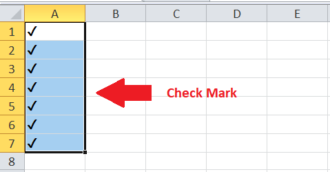
A check mark, also called a tick mark, refers to a sign or symbol used within Excel cells to denote positive responses like completed, done, yes, correct, etc. When the check mark is used within the cells, it is treated as text. Because it acts as a text format, we can adjust the appearance like color and size like any other text element. A check mark is also known by other names like the tick symbol and check symbol.

In Excel, check marks are typically used in two ways, interactive checkbox and tick symbol. When the check mark is used as an interactive checkbox, Excel allows us to select/ deselect an option by clicking on the rectangular box containing a tick sign inside it. Besides, a tick symbol (original check mark format) can be inserted within the cell alone or in combination with other elements like characters, symbols, etc.

Note: There is a difference between a check mark and a checkbox. The checkbox refers to the object that sits on top of the cell. According to this, a checkbox may not always be removed even after deleting the respective cell. However, the check mark follows the same Excel rules as the text format and can be copied or deleted along with the corresponding cell.

How to insert a check mark in Excel?

Excel provides several ways to access any existing feature or tool. Similarly, there are many other methods that help us easily insert check marks in one or more desired cells within an Excel worksheet. Following are some easy ways to insert a check mark or tick symbol in Excel, which works for all Excel versions, including Excel 2007, 2010, 2013, 2016, and above:

Method 1: By using the Copy-Paste

Like other elements, we can also copy a check mark in Excel. We can select and copy the check mark from the below box using the shortcut ‘Ctrl + C’.

After copying the above check mark, we need to go to the cell to paste it from the clipboard. Next, we need to double-click or press the F2 key on the cell to go to edit mode.

Lastly, we must paste the check mark using the shortcut ‘Ctrl + V’. This way, we can copy-paste the check mark in as many cells as required. However, it will be a time-taking method when we need to insert a checkmark in so many cells. Thus, we must look for other methods when inserting a check mark in huge workbooks.

Method 2: By using the Symbols Dialog Box

Another basic method to insert a check mark is choosing it from existing Excel symbols from the Symbols dialogue box. We need to perform the following steps:

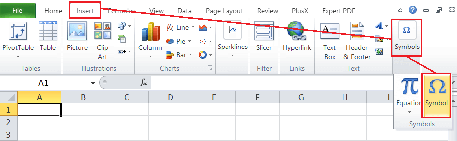
• First, we need to select the cells to insert a check mark. After that, we need to navigate the Insert tab on the ribbon.
• Next, we need to click the Symbol button under the section Symbols. This will launch the Symbols dialogue box.
  
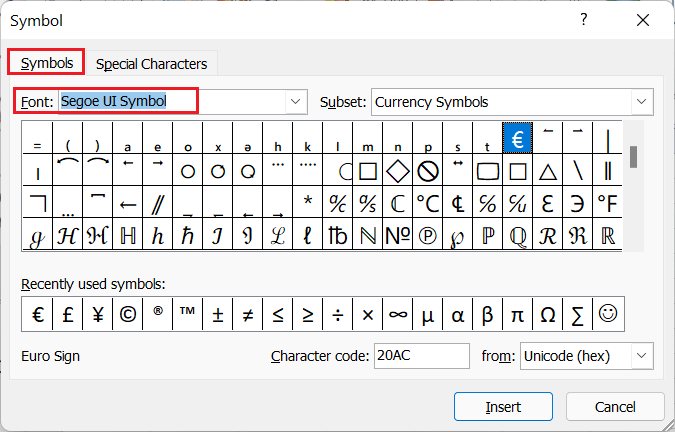
• In a dialogue box, we need to click on the drop-down next to Font and choose ‘Segoe UI Symbol’ from the list, as shown below:
  
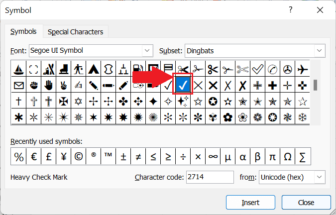
• We must scroll down the symbols section and locate the check mark, as shown below:
  
• Lastly, we must select the check mark and click the Insert button. The selected check mark is instantly inserted in all the desired cells within the worksheet.
  

Although it is a traditional method, it is also lengthy because finding a check mark from the Symbols dialogue box may take quite enough time.

Method 3: By using the Keyboard Shortcuts

Another method to insert a check mark includes using a keyboard shortcut. However, we cannot use the shortcut directly. We must follow the below steps:

• First, we need to select a cell to insert a check mark.
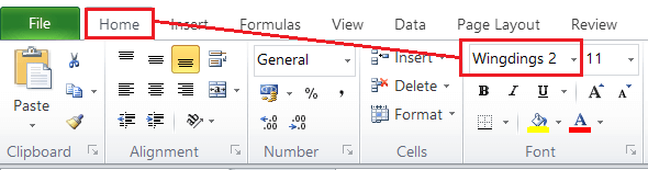
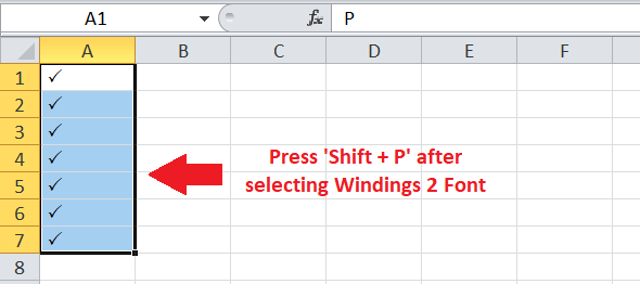
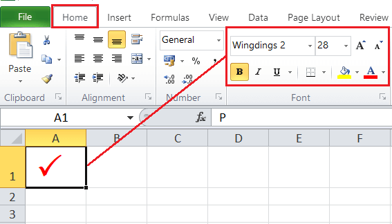
• Next, we need to click the drop-down list under the section Fonts. Here, we must select the font named ‘Wingdings 2’, as shown below:
  
• After selecting the specified font, we must use the keyboard shortcut ‘Shift + P’. This will immediately insert the check mark in the corresponding cell.
  
  Similarly, we can also choose the font ‘Wingdings’ and use the shortcut ‘Alt 0252’ to insert a check mark in the desired Excel cell. To insert a check mark into multiple cells, we can copy-paste it into other cells.

The keyboard shortcuts are one of the quickest methods to insert a check mark in Excel. However, this method is not suitable when we need to use a check mark with other text or numbers in the same cells. Since this method uses a specific font (Wingdings or Wingdings 2), we can use this method when we only need to insert a check mark in the cell.

Method 4: By using the CHAR Function

Excel has many built-in functions that help perform specific operations. Excel CHAR() function is a built-in function used to insert or display the desired character and special symbols within the Excel cells. This function can also be used to display a check mark in Excel.

To insert a check mark using the CHAR() function, we must perform the following steps:

• First, we need to select the Excel cells to insert a check mark.
• Next, we must use the below formula, which will help us to return a check mark symbol in the selected cell:

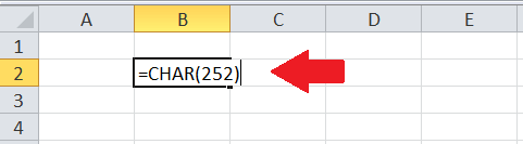
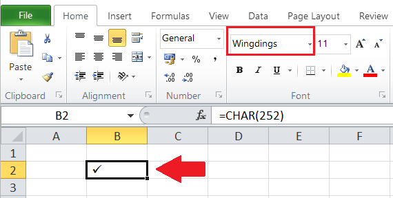
After typing the above function, we must press the Enter key.

• After that, we must again select the corresponding cell and change the font to Wingdings using the font drop-down under the Home tab. If we don’t change the font to Wingdings, Excel will display the ANSI character (ü). As soon as set the font to Wingdings, the ANSI character is changed to a check mark in the corresponding cell.
  

The advantage of using the CHAR() function to return a check mark is that we can combine it with other formulas and get a check mark based on certain rules or conditions.

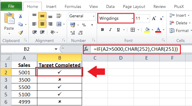
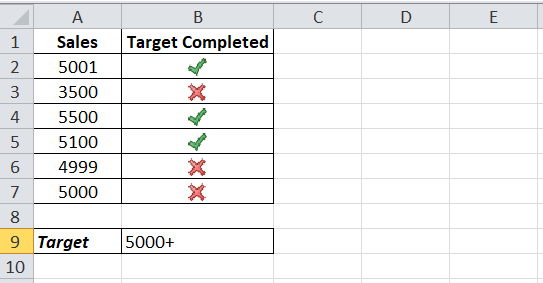
For example, let’s say we have the following sales data, and we want to display a check mark for sales that have exceeded 5,000, meaning the target has been met. In that case, we can use the formula like this:

In the above formula, 251 is the ASCII code of the cross symbol.

However, we must ensure that the respective cells have the font set to Wingdings.

It is important to note that this method is suitable only when we don’t need to insert any other character or symbol in the cell but a check mark. It is because the cells use the font Wingdings.

Method 5: By using the Conditional Formatting

Excel’s conditional formatting tool allows users to format the cells based on certain rules. This tool can be used to select pre-defined rules or create our own using the formula for the desired cells.

The conditional formatting tool is another easy-to-use method for inserting a check mark based on the corresponding cell values. The advantage of using the conditional formatting tool to insert a check mark is that we can adjust the check mark preferences (such as color, size, etc.) at once. As soon as certain conditions are met, the check mark symbol is inserted in respective cells with the specified formatting.

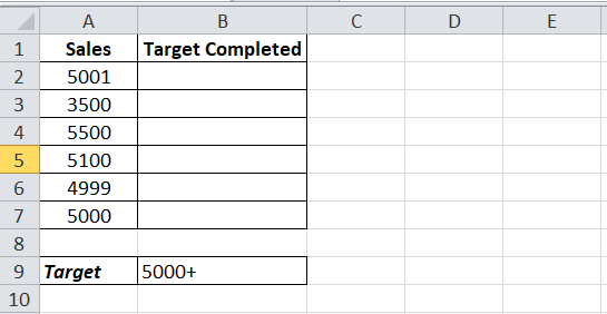
Let us again take the previous example sheet where we want to display a check mark for sales that have exceeded 5,000.

To insert a check mark in the above sheet, we must perform the following steps:

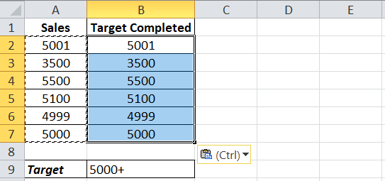
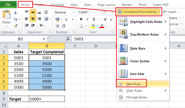
• First, we need to copy the values in the cells where we want to insert a check mark. Since we need to display check marks in column B, we copy the values from column A to the respective cells of column B, as shown below:
  
• Next, we must select all the effective cells of column B where we need to add a check mark.
• After that, we need to navigate the Home tab on the ribbon and choose the Conditional Formatting option. Here, we must click on the ‘New Rule’ option to open the ‘New Formatting Rule’ dialogue box.
  
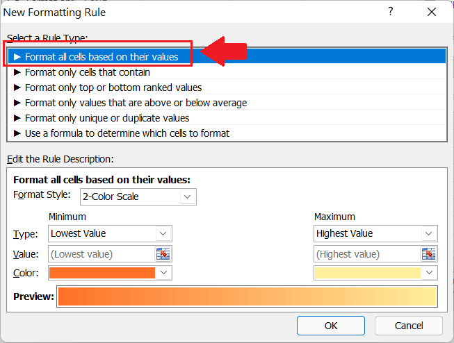
• We must choose ‘Format all cells based on their values’ under the ‘Select a Rule Type’ section in a dialogue box. Additionally, we need to click the drop-down box next to ‘Format Style’ under the ‘Edit the Rule Description’ section.
  
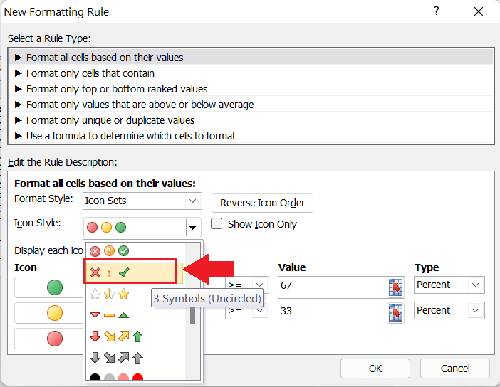
• In the drop-down list, we must click the ‘Icon Sets’ option to display additional options. Next, we must click the drop-down next to ‘Icon Style’ and choose the style containing a check mark, as shown below:
  
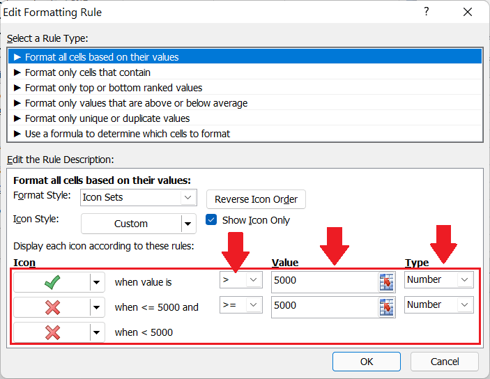
• After selecting the icon set, we must tick the ‘Show Icon Only’ box and set the other preferences like this:
  
  The above arrangement ensures displaying a check mark in cells with values of more than 5000. If the condition does not meet, the cross sign is displayed.
• Lastly, we must click the OK button. This will immediately insert the check marks (with color) in all the selected cells where the value is more than 5000, as shown below:
  

Similarly, we can also use the IF and CHAR functions combined in the conditional formatting tool and get the check mark in the desired cells.

Method 6: By using the Autocorrect

Excel has one distinct feature that automatically corrects certain misspelled words. For instance, if we type ‘back’ in an Excel cell, it automatically changes to ‘back’. It occurs because there is an existing list of misspelled words in Microsoft Office programs.

Using Autocorrect, we can insert a check mark in Excel very easily. It is the most useful method if we often need to insert a check mark in Excel. Although it is a quick-to-use method, we must configure this method once as discussed in the following steps:

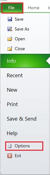
• First, we need to click on the File tab and select Options to open Excel options or settings.
  
• Next, we need to choose the Proofing option from the list and click the ‘AutoCorrect Options’ button, as shown below:
  
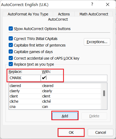
  This will open the Autocorrect dialogue box.
• We need to enter CMARK under the ‘Replace’ box and a check mark (✔) under the ‘With’ box in a dialogue box. After that, we must click the ADD button and the OK button.
  
  Now, whenever we need to insert a check mark, we can type CMARK in respective cells and press the Enter key. It will automatically change the text CMARK to a check mark.

While using this method, we should keep the following points in mind:

• The Autocorrect feature is case-sensitive. That means we must type the work CMARK (all CAPS) appropriately. If we enter Cmark or cmark, it will not be converted to a check mark.
• When we add to correct CMARK as a check mark, the changes get applied across all the Microsoft programs, such as Excel, Word, PowerPoint, etc.
• If there is an additional text or number before/ after the CMARK without a space in a cell, it will not get converted to a check mark. For example, if we type ‘100%CMARK’ or ‘CMARK100’, it will not change. However, ‘100% CMARK’ or ‘100% CMARK’ will change to the ‘100% ✔‘ or ‘100% ✔‘, respectively.

Method 7: By using the VBA (Double-click to insert Check Mark)

Excel VBA (Visual Basic for Applications) is one of the powerful features that allow us to perform advanced Excel operations. With a little VBA code, we can even create functionality where Excel will insert a check mark when we double-click on any cell within the sheet.

To insert a check mark using the VBA, we must perform the following steps:

• First, we need to open Excel VBA using the shortcut ‘Alt + F11’.
• Next, we need to right-click on the worksheet name from the Sheet tab. We must right-click only on those sheets where we want to use the check marks.
  

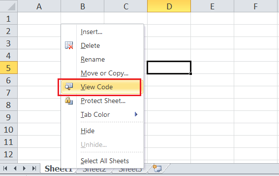
After that, we must select the ‘View Code’ option and copy-paste the following code in a Code window.

It will look like this:

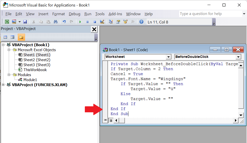
• Lastly, we must close the VBA window. Whenever we double-click on an Excel cell, the check mark is immediately inserted in the corresponding worksheet. We can follow the above steps for each sheet in the Excel workbook.

Formatting the Check Mark

The check mark in Excel can be formatted like the other texts used within the cells in the worksheet. We can change the size and color of the check mark as per our choice.

To format the check mark, we first need to select the cells with check marks, go to the Home tab, and navigate the Font section. Here, we can change the font size to increase or decrease the size of the size mark for the selected Excel cells. Likewise, we can select the font color button to change the color of the selected check marks.

Although it is an easy-to-use method of formatting the check marks, it can take time to format various check marks. Therefore, when formatting various check marks, it is always better to use the conditional formatting tool of Excel.

Removing the Check Mark

When we need to remove or delete check marks in Excel, we can use any of the following methods depending on the specific use case:

• When a check mark is used in a call or multiple cells without combination with other characters or symbols, we can select such cells and press the Delete key on the keyboard. To select contiguous or non-contiguous Excel cells, we can hold down the Shift or Ctrl key accordingly.
• When a check mark is used with the combination of other elements, we need to go through each corresponding cell individually. After going to a specific cell, we need to edit the cell content (press the F2 key to launch Edit Cell mode) and delete the checkmark using the Backspace key on the keyboard.
• When there are multiple cells where the check mark is combined with other elements, we must use Excel’s ‘Find and Replace’ tool. We need to select the effective cells (press ‘Ctrl + A’ to select the entire sheet), press ‘Ctrl + H’ to open Find and Replace, type a tick symbol next to the ‘Find what’ box, leave the ‘Replace with’ box empty and click the Replace All button.

---