Control system- Time response Analysis
The primary purpose of the time response analysis is to evaluate the system’s performance with respect to time. The time-response graph is shown below:
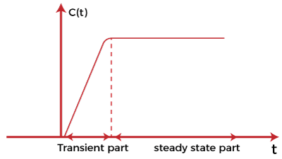
It comprises of two parts, transient part and the steady state part.
After applying an input to the control system, the output takes some time to reach the steady condition. The response during this stage is known as transient response and constitutes the transient part of the graph, as shown above. The graph when achieves the steady start after the transient part is known a steady part.
To describe a system, we need to develop the relationship between the inputs and output of the system that are the functions of time. The most common model used to describe such behavior is known as the differential equation. The analysis of the system can be done with the help of a differential equation by applying different inputs to it.
The common input signal is shown below:
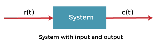
A test signal r(t) is applied as the input to the system that results in the response c(t). The input signal of a system can take many forms.
Note: The input and output are functions that vary with time.
Here, we will discuss the transient response, steady state response, and the standard signals of the control system.
Transient Response
It is a part of the time response that reaches 0 (zero) when the time becomes very large. In the graph analysis containing poles and zeroes, the poles lying on the left half of the s-plane gives the transient response. We can also say that it is a part of the response where output continuously increases or decreases. The transient response is also known as the temporary part of the response.
Or
Transient response is defined as the change in the response of the system from the equilibrium state.
For example,
The switching time of a bipolar transistor
The characteristics BJT or Bipolar Junction transistor depicts the transient nature.
Steady-state response
The response that comes after the transient response is called the steady-state response. In the graph analysis containing poles and zeroes, the poles on the imaginary axis give the steady-state response. We can also say that it is a part of the response where output remains constant. The output can also vary periodically with constant amplitude and frequency. The steady-state response is also known as the steady-state part of the response. It is a function of the input signal and hence also known as the forced response of the system.
Let’s discuss some examples where we will find the transient and steady-state terms of the given equation.
Examples
Example 1: 5 + 2e^-t
Solution:
Here, the transient part of the equation is 2e^-t because as t approaches to infinity, the term becomes 0. Hence, 2e^-t is the transient term. In the case of the first term 5, it will remain same when t approaches infinity. Hence, 5 is the steady-state term of the equation.
Example 2: 10 + 5e^t
Solution:
Here, the first term, 10, is the steady-state term of the equation because it will remain the same when t approaches infinity. In the case of the second term, 5e^t, the result is infinity when t approaches infinity. Hence, it is not a transient term. It is because something to the power infinity is always infinity.
So, there is only a steady-state term in the equation.
Standard signals
- Step Input signal
- Ramp input signal
- Sinusoidal input signal
- Impulse input signal
Step Input signal
For the positive value, the step input shows constant values of the time. It has zero value for the negative value of the time signal. The initial value of the signal is and the transition is in the form of step size with a constant value. If the constant value of the signal is 1, it is called step input signal, which is represented as:
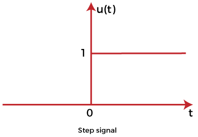
The value of the signal is:
0 for t=0 and
1 for t>0
The graph is a function of one variable named t.
Ramp input signal
The graph of the ramp input signal is in the shape of ramp. It depicts the linear increase that begins at some specific point. The value of the ramp signal shows the constant change with respect to time. The value of the signal is 0 for negative values. It means that it shows the output for positive inputs.
The ramp function is represented as:
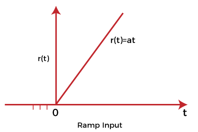
The value of the signal is:
At for t>0 and
0 for t<0
If the value of A is 1 when t>0. The signal is known as unit ramp signal.
Sinusoidal input signal
A sinusoidal input is one whose oscillations can be described by an equation in the form of sine. The response of the linear process to a sinusoidal is sinusoidal. The signal is given by:
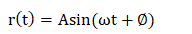
The sinusoidal signal in the control system is represented as:
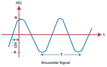
The sine wave starts from zero, covers positive value, reach zero, covers negative values, and again reaches zero, as shown above.
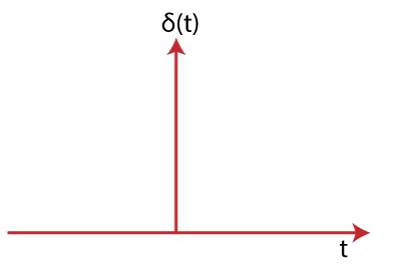
Impulse Input signal
The impulse signal is a type of high amplitude signal and has a very short duration. It means that the magnitude approaches infinity when the time reaches zero. Thus, we can say that the value of the signal is infinity at t =0. Otherwise, its value is 0.
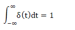
Its integration from -infinity to infinity is 1, as shown above.
It is a physical non-existing signal, which is defined based on the area concept. It is not based on the amplitude concept. The impulse input signal is represented as: