87

Data Reduction in Data Mining

Data mining is applied to the selected data in a large amount database. When data analysis and mining is done on a huge amount of data, then it takes a very long time to process, making it impractical and infeasible.

Data reduction techniques ensure the integrity of data while reducing the data. Data reduction is a process that reduces the volume of original data and represents it in a much smaller volume. Data reduction techniques are used to obtain a reduced representation of the dataset that is much smaller in volume by maintaining the integrity of the original data. By reducing the data, the efficiency of the data mining process is improved, which produces the same analytical results.

Data reduction does not affect the result obtained from data mining. That means the result obtained from data mining before and after data reduction is the same or almost the same.

Data reduction aims to define it more compactly. When the data size is smaller, it is simpler to apply sophisticated and computationally high-priced algorithms. The reduction of the data may be in terms of the number of rows (records) or terms of the number of columns (dimensions).

Techniques of Data Reduction

Here are the following techniques or methods of data reduction in data mining, such as:

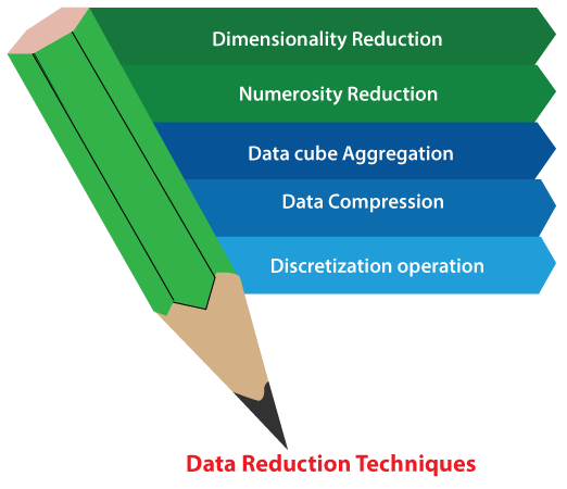
1. Dimensionality Reduction

Whenever we encounter weakly important data, we use the attribute required for our analysis. Dimensionality reduction eliminates the attributes from the data set under consideration, thereby reducing the volume of original data. It reduces data size as it eliminates outdated or redundant features. Here are three methods of dimensionality reduction.

1. Wavelet Transform: In the wavelet transform, suppose a data vector A is transformed into a numerically different data vector A’ such that both A and A’ vectors are of the same length. Then how it is useful in reducing data because the data obtained from the wavelet transform can be truncated. The compressed data is obtained by retaining the smallest fragment of the strongest wavelet coefficients. Wavelet transform can be applied to data cubes, sparse data, or skewed data.
2. Principal Component Analysis: Suppose we have a data set to be analyzed that has tuples with n attributes. The principal component analysis identifies k independent tuples with n attributes that can represent the data set.
   In this way, the original data can be cast on a much smaller space, and dimensionality reduction can be achieved. Principal component analysis can be applied to sparse and skewed data.
3. Attribute Subset Selection: The large data set has many attributes, some of which are irrelevant to data mining or some are redundant. The core attribute subset selection reduces the data volume and dimensionality. The attribute subset selection reduces the volume of data by eliminating redundant and irrelevant attributes.
   The attribute subset selection ensures that we get a good subset of original attributes even after eliminating the unwanted attributes. The resulting probability of data distribution is as close as possible to the original data distribution using all the attributes.

2. sNumerosity Reduction

The numerosity reduction reduces the original data volume and represents it in a much smaller form. This technique includes two types parametric and non-parametric numerosity reduction.

1. Parametric: Parametric numerosity reduction incorporates storing only data parameters instead of the original data. One method of parametric numerosity reduction is the regression and log-linear method.
   • Regression and Log-Linear: Linear regression models a relationship between the two attributes by modeling a linear equation to the data set. Suppose we need to model a linear function between two attributes.
     y = wx +b
     Here, y is the response attribute, and x is the predictor attribute. If we discuss in terms of data mining, attribute x and attribute y are the numeric database attributes, whereas w and b are regression coefficients.
     Multiple linear regressions let the response variable y model linear function between two or more predictor variables.
     Log-linear model discovers the relation between two or more discrete attributes in the database. Suppose we have a set of tuples presented in n-dimensional space. Then the log-linear model is used to study the probability of each tuple in a multidimensional space.
     Regression and log-linear methods can be used for sparse data and skewed data.
2. Non-Parametric: A non-parametric numerosity reduction technique does not assume any model. The non-Parametric technique results in a more uniform reduction, irrespective of data size, but it may not achieve a high volume of data reduction like the parametric. There are at least four types of Non-Parametric data reduction techniques, Histogram, Clustering, Sampling, Data Cube Aggregation, and Data Compression.
   • Histogram: A histogram is a graph that represents frequency distribution which describes how often a value appears in the data. Histogram uses the binning method to represent an attribute’s data distribution. It uses a disjoint subset which we call bin or buckets.
     A histogram can represent a dense, sparse, uniform, or skewed data. Instead of only one attribute, the histogram can be implemented for multiple attributes. It can effectively represent up to five attributes.
   • Clustering: Clustering techniques groups similar objects from the data so that the objects in a cluster are similar to each other, but they are dissimilar to objects in another cluster.
     How much similar are the objects inside a cluster can be calculated using a distance function. More is the similarity between the objects in a cluster closer they appear in the cluster.
     The quality of the cluster depends on the diameter of the cluster, i.e., the max distance between any two objects in the cluster.
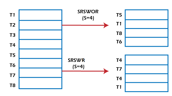
     The cluster representation replaces the original data. This technique is more effective if the present data can be classified into a distinct clustered.
   • Sampling: One of the methods used for data reduction is sampling, as it can reduce the large data set into a much smaller data sample. Below we will discuss the different methods in which we can sample a large data set D containing N tuples:
     1. Simple random sample without replacement (SRSWOR) of size s: In this s, some tuples are drawn from N tuples such that in the data set D (s<N). The probability of drawing any tuple from the data set D is 1/N. This means all tuples have an equal probability of getting sampled.
     2. Simple random sample with replacement (SRSWR) of size s: It is similar to the SRSWOR, but the tuple is drawn from data set D, is recorded, and then replaced into the data set D so that it can be drawn again.
        
     3. Cluster sample: The tuples in data set D are clustered into M mutually disjoint subsets. The data reduction can be applied by implementing SRSWOR on these clusters. A simple random sample of size s could be generated from these clusters where s<M.
     4. Stratified sample: The large data set D is partitioned into mutually disjoint sets called ‘strata’. A simple random sample is taken from each stratum to get stratified data. This method is effective for skewed data.

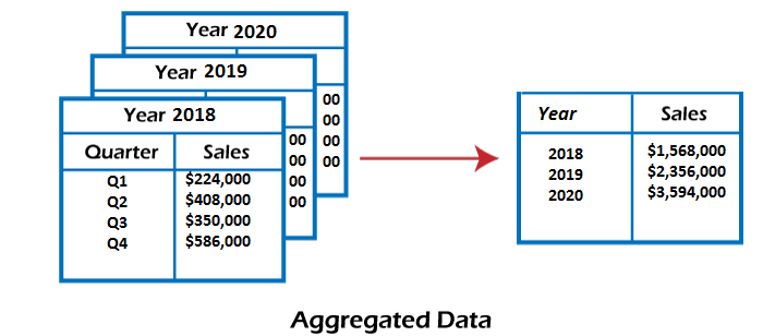
3. Data Cube Aggregation

This technique is used to aggregate data in a simpler form. Data Cube Aggregation is a multidimensional aggregation that uses aggregation at various levels of a data cube to represent the original data set, thus achieving data reduction.

For example, suppose you have the data of All Electronics sales per quarter for the year 2018 to the year 2022. If you want to get the annual sale per year, you just have to aggregate the sales per quarter for each year. In this way, aggregation provides you with the required data, which is much smaller in size, and thereby we achieve data reduction even without losing any data.

The data cube aggregation is a multidimensional aggregation that eases multidimensional analysis. The data cube present precomputed and summarized data which eases the data mining into fast access.

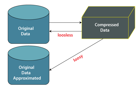
4. Data Compression

Data compression employs modification, encoding, or converting the structure of data in a way that consumes less space. Data compression involves building a compact representation of information by removing redundancy and representing data in binary form. Data that can be restored successfully from its compressed form is called Lossless compression. In contrast, the opposite where it is not possible to restore the original form from the compressed form is Lossy compression. Dimensionality and numerosity reduction method are also used for data compression.

This technique reduces the size of the files using different encoding mechanisms, such as Huffman Encoding and run-length Encoding. We can divide it into two types based on their compression techniques.

1. Lossless Compression: Encoding techniques (Run Length Encoding) allow a simple and minimal data size reduction. Lossless data compression uses algorithms to restore the precise original data from the compressed data.
2. Lossy Compression: In lossy-data compression, the decompressed data may differ from the original data but are useful enough to retrieve information from them. For example, the JPEG image format is a lossy compression, but we can find the meaning equivalent to the original image. Methods such as the Discrete Wavelet transform technique PCA (principal component analysis) are examples of this compression.

5. Discretization Operation

The data discretization technique is used to divide the attributes of the continuous nature into data with intervals. We replace many constant values of the attributes with labels of small intervals. This means that mining results are shown in a concise and easily understandable way.

1. Top-down discretization: If you first consider one or a couple of points (so-called breakpoints or split points) to divide the whole set of attributes and repeat this method up to the end, then the process is known as top-down discretization, also known as splitting.
2. Bottom-up discretization: If you first consider all the constant values as split-points, some are discarded through a combination of the neighborhood values in the interval. That process is called bottom-up discretization.

Benefits of Data Reduction

The main benefit of data reduction is simple: the more data you can fit into a terabyte of disk space, the less capacity you will need to purchase. Here are some benefits of data reduction, such as:

• Data reduction can save energy.
• Data reduction can reduce your physical storage costs.
• And data reduction can decrease your data center track.

Data reduction greatly increases the efficiency of a storage system and directly impacts your total spending on capacity.

---