79

Effective Root Searching Algorithms in Python

As Data Scientists and Computer Scientists, we often deal with root searching algorithms in our daily routines even if we did not realize it. These algorithms are designed to locate proximity to a specific value, local/global maxima, or minima.

We utilize a root searching algorithm in order to search for the proximity of a specific value, local/global maxima, or minima.

In mathematics, finding a root generally means that we are attempting to solve a system of equation(s) like f(X) = 0. This will make root searching algorithms a very efficient searching algorithm as well. All we have to perform is to define g(X) = f(X) – Y where Y is the search target and instead solve for X like g(X) = f(X) – Y = 0.

The Approaches are mainly categorized into two different families:

1. Bracket Approaches (For example, Bisection Algorithm)
2. Iterative Approaches (For example, Newton’s Method, Secant Method, Steffensen’s Method, and a lot more)

In the following tutorial, we will be understanding the implementation of some of these algorithms in the Python programming language and comparing them against each other. These algorithms are as follows:

1. Bisection Algorithm
2. Regula-Falsi Algorithm
3. Illinois Algorithm
4. Secant Algorithm
5. Steffensen’s Algorithm

Before we get started, let us assume that we have a continuous function f and would like to search for a value y. Thus, we are solving for the equation: f(x) – y = 0.

Understanding the Bisection Algorithm

Bisection Algorithm, also known for its discrete version (Binary search) or tree variant (Binary search tree), is an effective algorithm to search for a target value within a boundary. Due to that, this algorithm is also called a bracketing approach for finding a root of an algorithm.

Key Strength:

1. Bisection Algorithm is a robust algorithm that guarantees a reasonable convergence rate to the target value.

Key Weakness:

1. This algorithm requires knowledge of the estimated area of the root. For example, 3 ≤ π ≤ 4.
2. This algorithm works well; only one root is in the estimated area.

Suppose that we know that x is between f(p) and f(q), which forms the search bracket. The algorithm will check whether x is greater than or less than f((p + q) / 2), which is the mid-point of the bracket.

When searching a continuous function, probably, we will never be able to locate the exact value (For example, locating the end of ?). A margin of error is needed to check against the mid-point of the bracket. We can treat an error margin as an early stopping when the computed value is close to the target value. For example, if the error margin is 0.001%, 3.141624 is close enough to ?, approximately 3.1415926…

If the calculated value is close enough to the target value, the search is done, or else, we search for the value in the bottom half if x is less than f((p + q) / 2) and vice versa.

Let us now consider the following snippet of code demonstrating the same in Python.

Example:

Explanation:

In the above snippet of code, we have defined a function as bisectionAlgorithm that accepts some parameters like f, p, q, y, and margin where f is a callable, continuous function, p is a float value and lower bound to be searched, q is also a float value and upper bound to be searched, y is again a float value and the target value and margin is the margin of the error in absolute term and also a float value. We have then used the if conditional statement to check if the lower bound assigned to f(p) is greater than the upper bound assigned to f(q), for which the value of p and q is equal to q and p and lower and upper is equal to upper and lower. We have then used the assert keyword to debug the value of y. We have then used the while loop within which we have defined the value of r equals the mean of p and q. Inside this loop, we have also used the if-elif-else conditional statement to check if y_r assigned to f(r) – y is less than margin and returned r for the same.

Understanding the False Position Algorithm

Similar to the Bisection algorithm, the False Position Algorithm, also known as Regula Falsi, utilizes a bracketing approach. But unlike the Bisection Algorithm, it does not utilize a brute-force approach of dividing the problem space into half for every iteration. Instead, this algorithm iteratively draws a straight line from f(p) to f(q) and compares the intercept with the target value. However, there is no guarantee that the searching efficiency is always improved. For instance, the following diagram depicts how only the lower bound has been increased at a reducing rate, whereas the upper bound remains a stagnant bound.

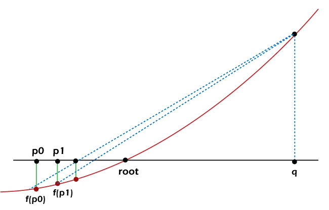
Figure 1: Stagnant bound slows down convergence

Key Strength:

1. This algorithm often shows faster convergence than the Bisection algorithm.
2. Regula Falsi benefits that as the bracket gets smaller, the continuous function will converge to a straight line.

Key Weakness:

1. Regula Falsi also shows slower convergence when the algorithm hits a stagnant bound.
2. This algorithm requires knowledge of the approximate area of the root. For example, 3 ≤ π ≤ 4.

The significant difference in the implementation between Regula Falsi and Bisection Algorithm is that r is no longer the mid-point between p and q; however, instead is being estimated as:

Let us consider the following snippet of code demonstrating the same:

Example:

Explanation:

In the above snippet of code, we have defined a function as regulaFalsiAlgorithm that accepts some parameters like f, p, q, y, and margin where f is a callable, continuous function, p is a float value and lower bound to be searched, q is also a float value and upper bound to be searched, y is again a float value and the target value and margin is the margin of the error in absolute term and also a float value. We have then used the assert keyword to debug the value of y. We have then used the while loop within which we have defined the value of r. Inside this loop, we have also used the if-elif-else conditional statement to check if y_r assigned to f(r) – y is less than margin and returned r for the same.

Understanding the Illinois Algorithm (Modified Regula Falsi)

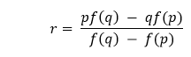
In order to get past the stagnant bound, we can insert a conditional rule for when a bound remain stagnant for two rounds. Taking the previous example, as q has not moved for two rounds, and that r is not close to the root x yet, in the next round, the line will be drawn to f(q) / 2 instead of f(q). The same will be implemented for the lower bound if, the lower bound is the stagnant bound.

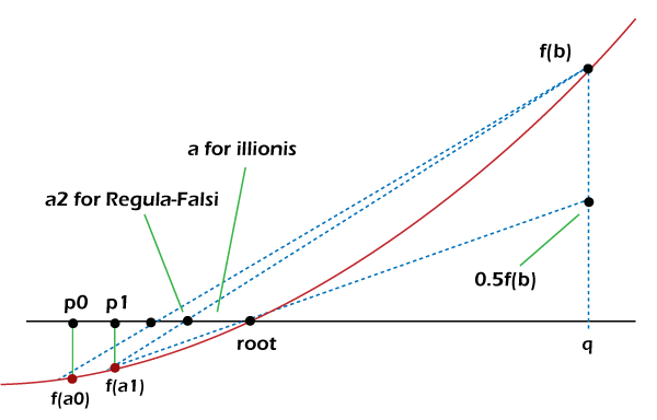
Figure 2: Illinois Algorithm avoid prolonged stagnant bound for faster convergence.

Key Strength:

1. Illinois Algorithm shows faster convergence than both the Bisection algorithm and the Regula Falsi algorithm.
2. We can avoid stagnant bound by halving the distance of the stagnant bound to the target value.

Key Weakness:

1. This algorithm also shows slower convergence when the algorithm hits a stagnant bound.
2. This algorithm requires knowledge of the estimated area of the root. For example, 3 ≤ π ≤ 4.

Example:

Explanation:

In the above snippet of code, we have defined a function as illinoisAlgorithm that accepts some parameters like f, p, q, y, and margin where f is a callable, continuous function, p is a float value and lower bound to be searched, q is also a float value and upper bound to be searched, y is again a float value and the target value and margin is the margin of the error in absolute term and also a float value. We have then used the assert keyword to debug the value of y. We have then defined a variable as stagnant equals to zero. We have then used the while loop within which we have defined the value of r. Inside this loop, we have also used the if-elif-else conditional statement to check if y_r assigned to f(r) – y is less than margin and returned r for the same.

Understanding the Secant Method (Quasi-Newton’s Method)

Till now, we have been implementing the bracket approaches. What if we don’t know the location of the brackets? In such cases, the secant method can be helpful. The Secant method is an iterative algorithm that begins with two values and tries to converge towards the target value. While we can get better performance while the algorithm convergence and don’t require knowledge of the rough root location, we may run into the risk of divergence if the two initial values are too far away from the real root.

Key Strength:

1. The Secant method does not need a bracket consisting of the root.
2. This method does not need knowledge of the estimated area of the root.

Key Weakness:

1. Unlike all the earlier methods, the Secant method does not guarantee convergence.

The Secant method begins by checking two user-defined seeds. Suppose we want to find a root for x² – math.pi = 0 starting with x_0 = 4 and x_1 = 5; our seeds will be 4 and 5, respectively. (Note: This process is similar to searching for x like x² = math.pi)

Figure 3: Secant’s method of locating x3 based on x1 and x2

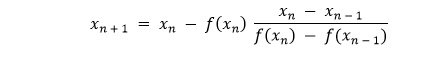
We then locate the intercept with the target value x_2 by drawing a straight line through f(x_0) and f(x_1) what we have done in the Regula Falsi algorithm. If f(x_2) is not close enough to the target value, we must repeat the step and locate x_3. In general, we can calculate the next x using the following formula:

Let us consider the following snippet of code demonstrating the same:

Example:

Explanation:

In the above snippet of code, we have defined a function as secantAlgorithm that accepts some parameters like f, x0, x1, y, iterations, and margin where f is a callable, continuous function, x0 and x1 are the float values and the initial seeds, y is again a float value, and the target value, iterations is a integer value and stores the value of maximum number of iterations to avoid indefinite divergence, and margin is the margin of the error in absolute term and also a float value. We have then used the assert keyword to check if the value of x0 is not equals to the value of x1. We have then used the if conditional statement to check if the y0 assigned to f(x0) – y is less than the margin variable and returns the x0 variable for the same. We have again used if conditional statement to check if the y1 assigned to f(x1) – y is less than the margin variable and returns the x1 variable for the same. At last, we have used the for-loop to iterate through the values stored in the iterations variable and defined formula to find the roots. Within the loop, we have again used the if conditional statement and return x2.

Understanding the Steffensen’s Method

The Secant’s method further improves the Regula Falsi algorithm by eliminating the requirements of a bracket consisting of a root. Let us recall that the straight line is only a naïve value of the tangent line (that is, the derivative) of two x values (or upper and lower bound in the case of Regula Falsi and Illinois algorithm). This value will be perfect as the search converges. In Steffensen’s algorithm, we will attempt to replace the straight line with a better value of the derivative for further improving Secant’s method.

Key Strength:

1. Steffensen’s method does not need a bracket consisting of the root.
2. This method also does not need knowledge of the estimated area of root.
3. This method shows faster convergence than Secant’s method if possible.

Key Weakness:

1. Steffensen’s method does not give assurance on convergence if the initial seed is too far away from the real root.
2. The continuous function will be evaluated twice that of Secant’s method to better calculate the derivative.

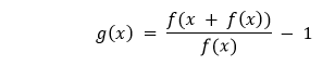
We can estimate the derivative better with the help of Steffensen’s Algorithm by computing the following based on the user-defined initial seed x0.

Which is equivalent to the following where h = f(x):

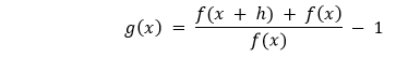
Take a limit of h to 0 and we will get a derivative of ?(?).

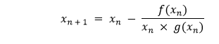
We will then use the generalized evaluated slope function to locate the next step following the same procedure as Secant’s method:

Let us consider the following snippet of code demonstrating the same:

Example:

Explanation:

In the above snippet of code, we have defined a function as secantAlgorithm that accepts some parameters like f, x0, x1, y, iterations, and margin where f is a callable, continuous function, x0 and x1 are the float values and the initial seeds, y is again a float value, and the target value, iterations is a integer value and stores the value of maximum number of iterations to avoid indefinite divergence, and margin is the margin of the error in absolute term and also a float value. We have then used the assert keyword to check if the initial seed is not equal to zero. We have then used the if conditional statement to check if the yx assigned to f(x) – y is less than the margin variable and returns the x variable for the same. At last, we have used the for-loop to iterate through the values stored in the iterations variable and defined formula to find the roots. Within the loop, we have again used the if conditional statement and return x.

Conclusion

In the above tutorial, we have understood the strength, weakness, and the implementation of the following five algorithms used to search root.

1. Bisection Algorithm
2. Regula Falsi Algorithm
3. Illinois Algorithm
4. Secant’s Algorithm
5. Steffensen’s Algorithm

Let us now consider the following table showing the comparison of algorithms we have implemented.

	Bisection Algorithm	Regula Falsi Algorithm	Illinois Algorithm	Secant’s Algorithm	Steffensen’s Algorithm
Approach	Bracket	Bracket	Bracket	Iterative	Iterative
Convergence	Guaranteed	Guaranteed	Guaranteed	Not Guaranteed	Not Guaranteed
Knowledge of Approximate Location of Root	Required	Required	Required	Not Required	Not Required
Number of Initial Seeds	2	2	2	2	1
Risk of Slow Convergence	Not Available	Stagnant Bound	Not Available	Initial Seed not close enough to Root	Initial Seed not close enough to Root
Method of Reducing Problem Space	Brute-force Halving	Approximate Derivate with Finite Difference	Approximate Derivate with Finite Difference	Approximate Derivate with Finite Difference	Approximate Derivate with Finite Difference
Speed of Convergence	Linear	Linear	Super-linear	Super-linear	Quadratic

Once we get comfortable with these algorithms, many other root-finding algorithms to explore have not been covered in this tutorial. Some of them are Newton-Raphson’s Method, Inverse Quadratic Interpolation, Brent’s Method, and more. Keep exploring and add the above algorithms to the arsenal of tools.

---