Excel ABS Function
Microsoft Excel is all about managing data, especially numbers. We know that the primary thing with numbers is that they can either be positive or negative. But various data should be essentially positive. Excel has provided an inbuilt function to cater to these requirements, i.e., ABS Function.
This tutorial will cover the definition of Excel ABS Function, its syntax, parameters, return type, steps to implement ABS function in your worksheet, and many more!
What is ABS Function?
The ABS or Absolute function in Excel returns the absolute value of the given number. In simple terms, we can say that the ABS function eliminates the minus symbol (-) from the specified number, therefore making it a positive number.
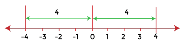
The absolute value of any given number is defined as the distance of that number from 0 on a number line, nevertheless of its direction (positive or negative). In mathematics, the absolute value of a number ‘a’ is represented as |a| unlike in the given below examples:
|-4| = 4
Though Microsoft Excel does not directly provide any absolute value symbol, it has introduced a special function for getting an absolute value known as the ABS function. While using the ABS or Absolute Function, we will get one of the below given visual and outputs:
- If the specified absolute number is positive, the output will be the number itself.
- If the specified absolute number is negative, the output will be the number without its negative sign.
- If the specified absolute number is zero, the output is also 0.
Note. Excel absolute value should not be mistaken with Excel absolute cell reference. Both are different concepts. The absolute function eliminates the minus symbol (-) from the specified number whereas an absolute reference is a special form that remains unaffected while copying the same formula to other cells.
Syntax
Parameter
Number (required): This parameter represents the number for which you want to fetch the absolute value.
Return
The Excel ABS function returns the absolute value for the specified number. If the specified number is non-numeric, this function returns a #VALUE! error.
Examples
Example 1: Using Excel ABS function convert the negative number to positive number.
In cases where you require to convert negative numbers to positive numbers quickly, the Excel ABS function is a handy option. Follow the below-given steps to change a negative number to a positive number:
Step 1: Insert two helper columns
We will add two columns one named with ‘Difference’ in cell D3 and another named with ‘Absolute Difference’ in cell E3.
Refer to the given below image:
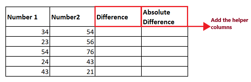
- In the difference helper column we will simply use the minus sign to calculate the difference of both the cells
- In the ABS Difference helper column we will apply the Excel ABS function and fetch the absolute value.
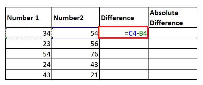
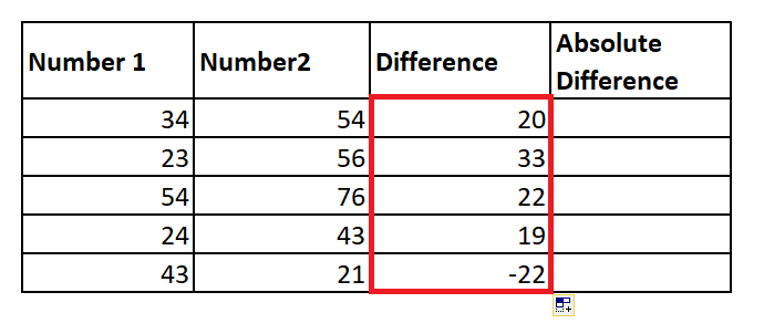
STEP 2: Subtract number1 from number2
- In the difference column type the equal sign (=) and subtract number2 from number1.
- Press the enter key to fetch the result.
- Select the cell where you have typed the formula. Take your mouse cursor towards the end of the rectangular box. You will notice the cursor will change into a small thin black cross. Drag it over the cells you want to auto-fill.
- You will have the following outputs.
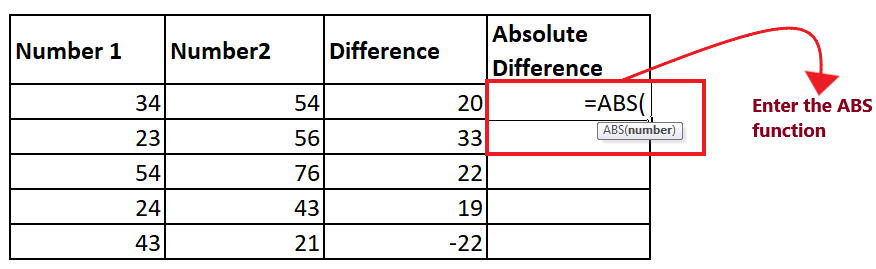
STEP 3: Insert the ABS function
In the next row, start your function with the equal to (=) sign followed by the abs function. The formula will be as follows: =ABS(
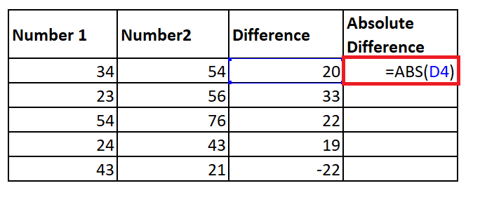
STEP 4: Insert the number parameter
Refer to the number parameter for which you want to find the absolute number. Since here, we have to find the absolute value of the Difference column. So we will refer to the D4 cell. The formula will be as follows: =ABS(D4)
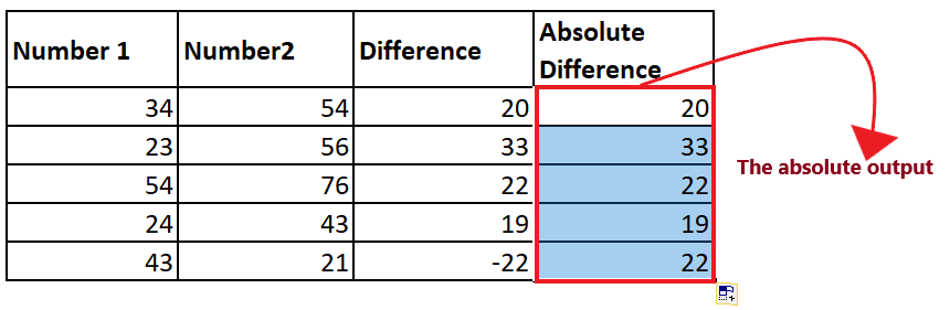
STEP 5: Copy the formula across all the cells
- Select the cell where you have typed the formula. Take your mouse cursor towards the end of the rectangular box. You will notice the cursor will change into a small thin black cross. Drag it over the cells you want to auto-fill.
- The abs function will successfully fetch the absolute difference for the specified numbers.
Refer to the given below image:
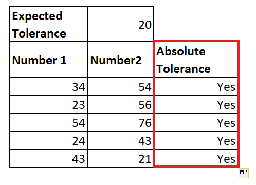
Example 2: Using the Excel ABS function find whether a given value (number or percentage) is within expected tolerance or not.
The ABS function is also commonly used to find whether a specified value is within expected tolerance or not. Follow the below-given steps to check whether the number is in between the expected tolerance or not:
Step 1: Insert the absolute helper column
We will add the helper columns named with ‘Absolute Tolerance’ in cell D3.
Refer to the given below image:
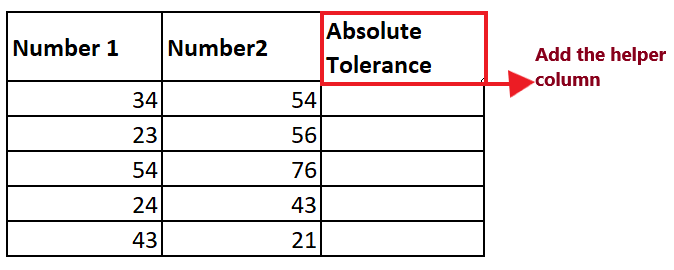
In the ABS Difference helper column, we will apply the Excel combination of IF and ABS function to check whether the number is in between the expected tolerance.
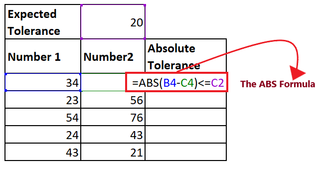
STEP 2: Insert the ABS function
- Start your function with the equal to (=) sign followed by the abs function. The formula will be as follows: =ABS(
- Subtract number1 from number2 and fetch the absolute value of the difference. The formula will be as follows: =ABS(B4-C4)
- Next we will check if the fetch value is less than or equal to the specified tolerance. The formula will be as follows: =ABS(B4-C4)<=C2
It will look like the below image:
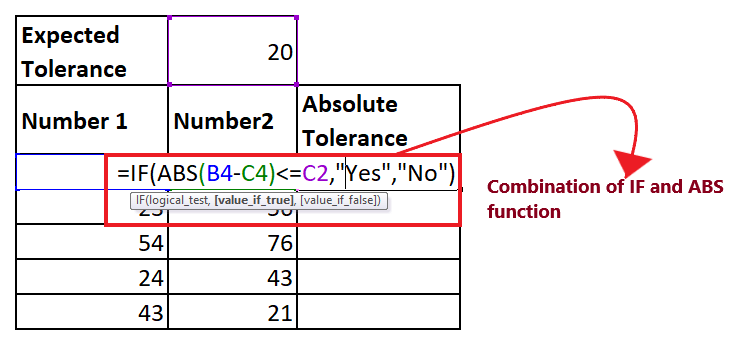
STEP 3: Apply the IF function
- To check whether the absolute output is within the tolerance range we use a combination of IF along with ABS function.
- For instance, in our case we return “Yes” if the difference is within tolerance, “No” otherwise:
=IF(ABS(A2-B2)<=C2, “Yes”, “NO”)
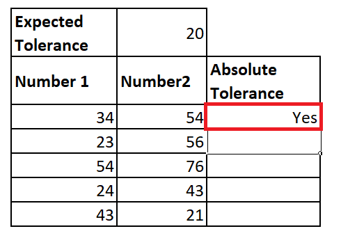
STEP 4: Formula will return the output
The above function will return Yes if tolerance if greater than C2 else it will return Fail. In our case, the output is “Yes”.
STEP 5: Copy the formula across all the cells
- Select the cell where you have typed the formula. Take your mouse cursor towards the end of the rectangular box. You will notice the cursor will change into a small thin black cross. Drag it over the cells you want to auto-fill.
- The abs function will successfully fetch the absolute tolerance for the specified numbers.
Refer to the given below image:
STEP 5: Explanation of the formula
Inside the IF formula, both the specified numbers are subtracted. The return output could be positive or negative, depending on the actual value. Therefore we have implemented the ABS function to convert the output to a positive number for all the cases. The fetched positive number is then compared to the allowed tolerance as a logical test inside IF. If the number is less than or equal to the specified tolerance, the function returns “OK”. If it doesn’t meet the specification, it returns “Fail”.
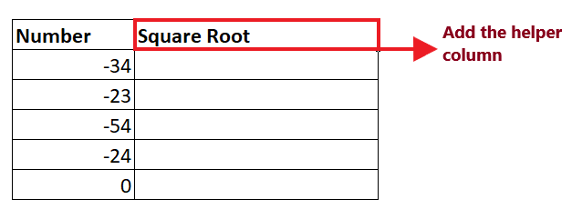
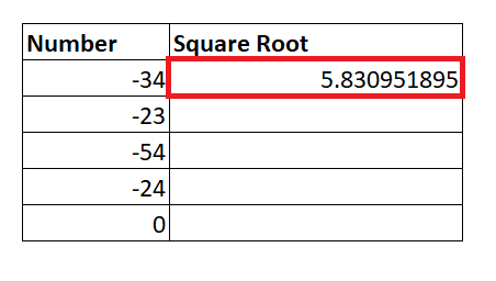
Example 3: Calculate the Square root of negative number using the Abs function.
We will use the SQRT function to calculate the square root of a negative number. But the SQRT function only works for positive numbers. What if the user wants to find the square of a negative number?
Follow the below-given steps to calculate the square root of a negative number:
Step 1: ADD the helper column
We will add the helper column helper with ‘square root’ in cell C3. In this column, we will use a combination of SQRT and ABS functions to find the square root of a negative number.
Refer to the given below image:
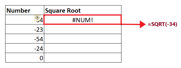
STEP 2: Implement the SQRT Function
- Excel provides an inbuilt function SQRT that helps calculate the square root of a number.
- If you pass a positive number in this parameter, it will return the output, but if you pass a negative number in this function, it will return a #NUM! error as shown below:
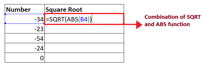
STEP 3: Insert the ABS function
- To handle a negative number like a positive number, you can use the combination of SQRT and ABS function.
- Insert the ABS function insert the SQRT function and add the number parameter as shown below:
STEP 4: Excel will return the output
The above formula will return the square root of the negative number.
STEP 5: Copy the formula across all the cells
- Select the cell where you have typed the formula. Take your mouse cursor towards the end of the rectangular box. You will notice the cursor will change into a small thin black cross. Drag it over the cells you want to auto-fill.
You will have the following output.

How to sum absolute values in Excel
While working with Excel sometimes we want to get an absolute sum of all numbers, use one of the following formulas:
Array formula:
The ABS function in Excel can also be used with the SUMPRODUCT function to count absolute variances that satisfies some particular conditions.
Regular formula:
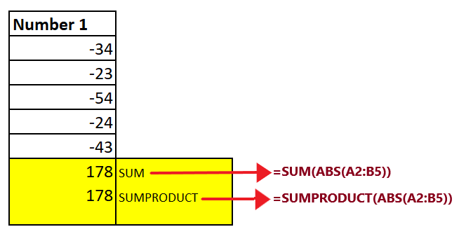
For example, Let’s suppose we have a dataset our worksheet in B2:C5 cells, using the ABS function we will find the sum absolute values.
Formula to obtain the absolute value using the SUM function:
=SUM(ABS(A2:B5))
Press the Ctrl+ Shift+ Enter and you will have the following output.
Formula to obtain the minimum absolute value:
=SUMPRODUCT(ABS(A2:B5))
Press the Ctrl+ Shift+ Enter and you will have the following output.
As you can see in the below image, both the sum formulas are returning an absolute value:
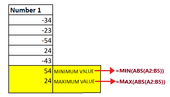
How to find the maximum/minimum absolute value in Excel
You can also fetch the minimum and maximum absolute value in Excel using the combination of ABS and other Excel formula.
Formula of Maximum absolute value is as follows:
Formula of Minimum absolute value is as follows:
For example, Let’s suppose we have a dataset our worksheet in B2:C5 cells, using the ABS function we will find the Min and MAX absolute value.
Formula to obtain the maximum absolute value:
=MAX(ABS(A2:B5))
Press the Ctrl+ Shift+ Enter and you will have the following output.
Formula to obtain the minimum absolute value:
=MIN(ABS(A2:B5))
Press the Ctrl+ Shift+ Enter and you will have the following output.
You can take the advantage of the ABS function and process a range of data by nesting it into the array argument of the INDEX function. We can incorporate a combination of MAX function, INDEX function and ABS Function to obtain the maximum absolute output. Below is the given formula:
=MAX(INDEX(ABS(B2:C5),0,0))
We can incorporate a combination of MIN function, INDEX function and AB Function to obtain the minimum absolute output. Below is the given formula:
=MIN(INDEX(ABS(B2:C5),0,0))
Explanation
The above formulas return the minimum and maximum values because of INDEX formula. When we set the argument (row_num and column_num) of INDEX function 0 (or omit them), Excel returns the entire array instead of any individual value.