Excel Filter Function
The filter option is one of the frequently used features of Excel. Users commonly filter out the data using Auto Filter and in more complex data problems with Advanced Filter. Though these methods are fast and powerful, they are not dynamic. In simple terms, these methods are not updated automatically whenever there is any change in the original data. Therefore, you would have to remove the filter, change the data, and apply the filter again. This way, it is very time-consuming.
To prevent this drawback, Excel introduced the long-awaited alternative, i.e., the FILTER function in Excel 365. Unlike the previous methods, the Excel FILTER() function recalculates the data automatically with each worksheet change, easing your task, as now you only need to set up your filter once!
What is Filter Function?
The Excel FILTER function is used to filter the range or array of values based on the given criteria. This function returns an output containing an array of values from the original range that automatically spills into a range of cells, beginning from the excel cell where you enter the Filter function.
The FILTER function generates dynamic output. When the values in the original data change or if the size of the original data array alters, the FILTER function automatically updates the output. Further, the result from this function will “spill” onto the Excel sheet into various cells. The Filter function belongs to the group of Dynamic Arrays functions.
The primary role of the FILTER function is to extract the matching values from a given data set by supplying one or more logical tests (or criteria). Logical tests are applied using the ‘include’ parameter, and it can hold various types of formula criteria. For instance, FILTER can match data in a specific employee sheet and fetch all the employee names whose sales figures are less than 350000 INR (or any other specified threshold value).
Note: The FILTER() function is only available with the latest Excel versions, i.e., Office 365 subscriptions and Excel 2021. Therefore, this function is not supported in the previous versions, unlike Excel 2019, Excel 2016, and all other earlier versions.
Syntax
Parameters
- Array (required) – This parameter represents the range of cells or the array of values in Excel worksheet that you wish to filter.
- Include(required) – This parameter represents the criteria that you want to apply to your array. It can be provided as a Boolean array (TRUE and FALSE values).
For example, (B2:B6)>2 is a Boolean criterion where we have mentioned that the filter function should only extract data from range B2: B6 if their value is greater than 2. - If_empty(optional) – This argument represents the value to return when none of the criteria is met. Typically it includes a customized user message such as “No values found”, but you can supply other values as well. You don’t pass any value in this parameter, it will take an empty string (“”) as the default value and will return nothing.
Points to Remember for Excel FILTER function
Below given are some important points that will help you to apply the FILTER function in your Excel worksheets effectively:
- The FILTER function analyzes the criteria and, based on the criteria it automatically spills the output horizontally or vertically, depending on how your source data is arranged in the Excel worksheet. So, always remember to have sufficient empty cells down and to the right of the cells; otherwise, Excel will throw a #SPILL error.
- The FILTER function generates dynamic output, meaning the values in the original data change, or if the size of the original data array changes, the FILTER function will automatically update the output. However, the range provided for the parameter ‘array’ is not updated when new values are added to your original data. But if you want to resize the array argument automatically, you must convert it to an Excel table or create a dynamic named range.
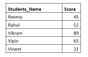
Example 1: Filter out the student’s name from the below Excel table, where student’s score is greater than 50.
Follow the below steps to solve the above problem:
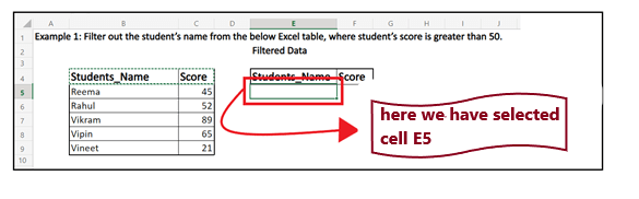
Step 1: Select a cell
Select a cell where you want to put your filter data. Always make sure to have enough empty cells towards the right and bottom of your selected cell, as it could value multiple values based on your original data.
As you can see in the below image, here we have selected cell E5.
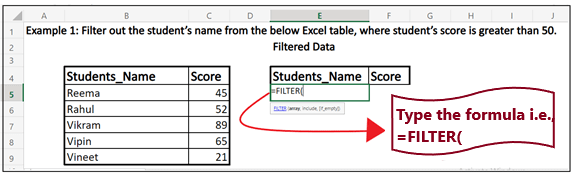
Step 2: Type the formula i.e., =Filter(
After you select the blank cell (E5), just type the formula: = Filter(
It will look similar to the below image:
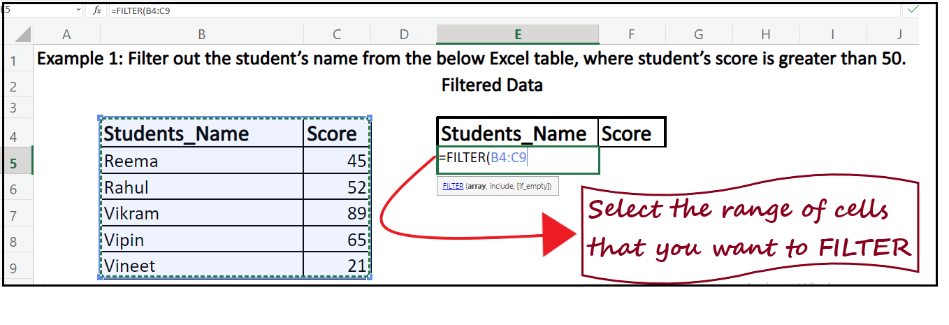
Step 3: Enter the range of cells or array you wish to transpose
The next step is to type (or select) the range of the cells or array you want to filter. Although instead of typing you can point and drag your mouse cursor to select the group of original cells.
In this example, the original cells are positioned from B4 to 9. Therefore our formula becomes: =FILTER (B4: C9. It will look similar to the below image:
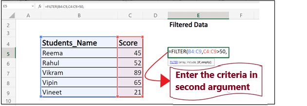
Step 4: Enter the criteria
We will move to the next argument (criteria) so firstly we will put a comma (,). Here, we need to filter the names of students whose score is greater than 50. So our criteria is Score (range of cells) > 50.
In this example, the score cells are positioned from C4 to C9. Therefore our formula becomes: =FILTER (B4: C9, C4:C9 > 50. It will look similar to the below image:
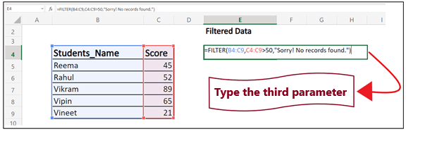
Step 4: Fill value in the third argument (though this step is optional)
In this argument we will type a customized user message such as “Sorry! No records found”, but you can supply other values as well. If you don’t pass any value in this parameter, it will take an empty string (“”) as the default value and will return nothing.
Therefore our formula becomes: =FILTER (B4: C9, C4:C9 > 50, “Sorry! No records found”). It will look similar to the below image:
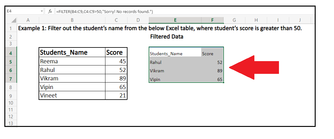
Step 5: Press enter and Excel will give the filtered output
As soon as you press the enter button, you will have the filtered records in front of you.
In our case, we have three fields where the score is greater than 50. And we have received the same three fields.
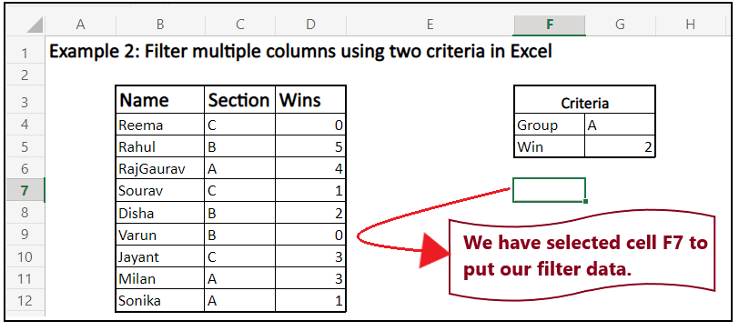
Example 2: Filter multiple columns using two criteria (given below) in Excel.
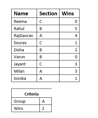
This is the extension of our basic Filter() function. In this example we will learn how to apply two criteria on two different columns and filter out our data.
Follow the below steps to solve the above problem:
Step 1: Select a cell
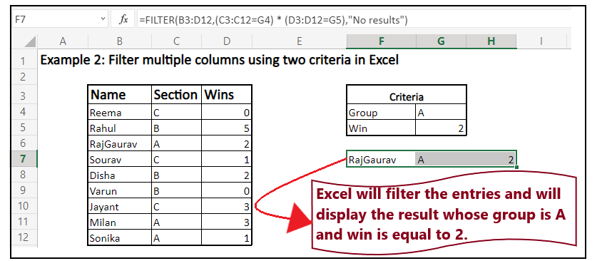
Select a cell where you want to put your filter data. As you can see in the below image, here we have selected cell F7.
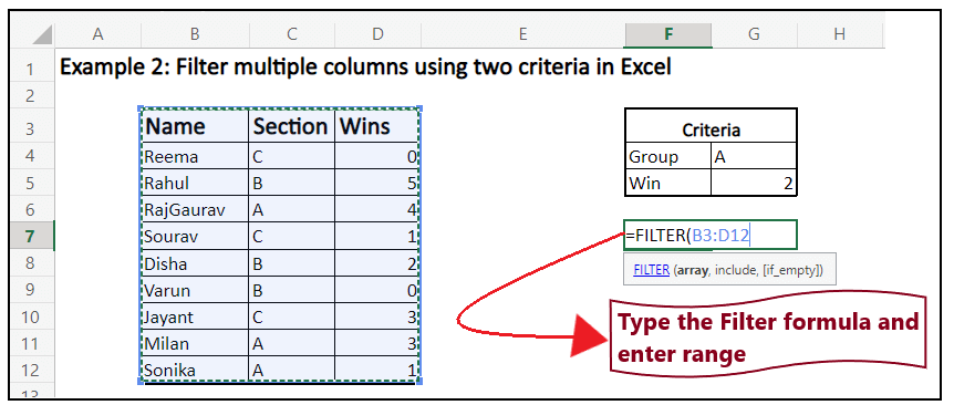
Step 2: Type the formula and enter the range of cells
The next step is to type the Filter function and select the range of the cells you want to filter. In our case, the original cells are positioned from B3 to D12. Therefore our formula becomes: =FILTER (B3: D12.
It will look similar to the below image:
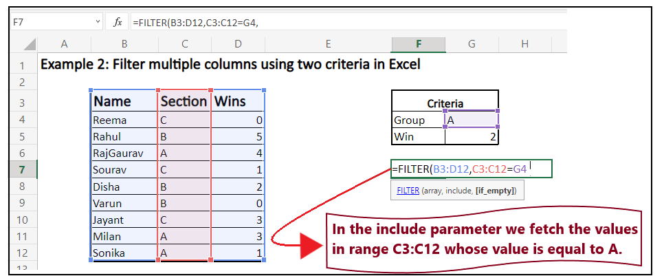
Step 3: Apply the first criteria
Firstly we will set up the criteria to specify the group. For this, we have entered the targeted group name in cell G4 (criteria1). Therefore we will check if any value in between range C3: C12 is equal to G4 or not. The formula will be as follows:
=FILTER(B3:D12, (C3:C12=G4),
Step 4: Apply the second criteria and combine them using AND (*) operator
In the second criteria, we will specify the minimum required number of wins in cell G5 (criteria2). Again, we will check if the values in between D3: D12 are equal to G5. Later combine criteria 1 and 2 using AND operator, and we will use the logical expression for AND, i.e., ‘*’.The formula will be as follows:
=FILTER(B3:D12, (C3:C12=G4)*(D3:D12= G5), “no results”)
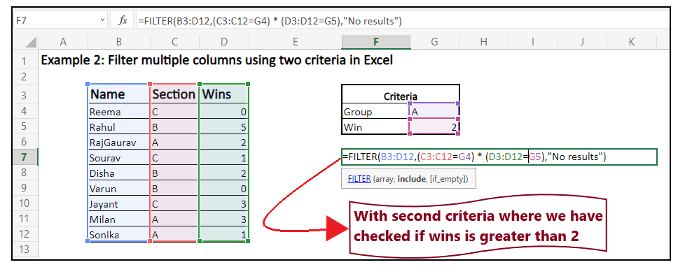
NOTE: In case of ‘AND’ or ‘*’ logical operator, the data entries will be extracted only if both the criteria must be TRUE. If for any entry the criterion is FALSE, they will be filtered out.
Step 5: Press the enter button to fetch the output
Excel will filter the entries for you and fetch a list of candidates from group A who have secured more than 2 wins.
It will look similar to the below image:
Example 3: Excel Filter function with multiple criteria (using AND & OR logic)
You can also implement the Filter function to obtain data with multiple criteria. Often when we want to apply multiple criteria in our formulas, we use OR and AND conditions. Unlike in the previous example, we have used logical expression for AND (*), but you also need to add (using + logical expression) them in many cases.
In the case of ‘AND’ or ‘*’ logical operator, the data entries will be extracted only if both the criteria must be TRUE. If for any entry the criterion is FALSE, they will be filtered out.
In the case of the ‘OR’ or ‘+’ logical operator, the resulting array will return 0 if both criteria are not met and appear False. If any of the specified criteria is TRUE, it will extract the data for that entry.
Follow the below steps to solve the above problem:
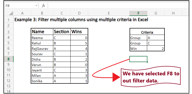
Step 1: Select a cell
Select a cell where you want to put your filter data. As you can see in the below image, here we have selected cell F8.
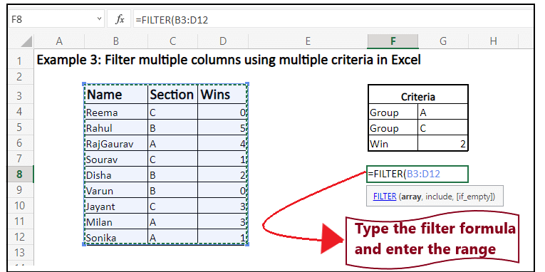
Step 2: Type the formula and enter the range of cells
Next, we will type the Filter function and enter the range. In our case, the original cells are positioned from B3 to D12. Therefore our formula becomes: =FILTER (B3: D12.
It will look similar to the below image:
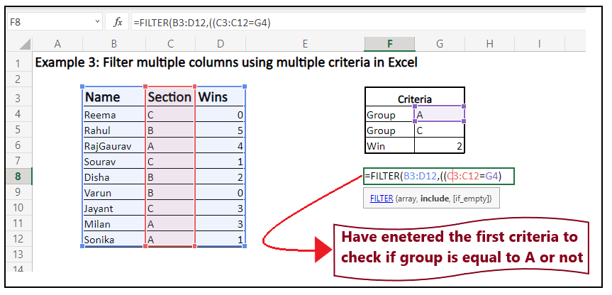
Step 3: Apply the first criteria
Firstly we will set up the criteria to specify the group. For this, we have entered the targeted group name in cell G4 (criteria1). Therefore we will check if any value in between range C3: C12 is equal to G4 or not. The formula will be as follows:
=FILTER(B3:D12,((C3:C12=G4)
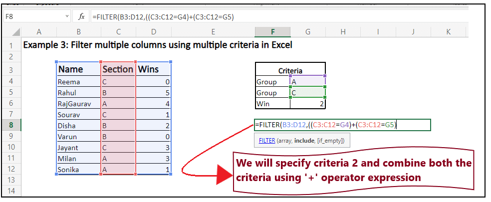
Step 4: Apply the second criteria and combine first and second criteria using ‘+’ (OR) operator.
Next we will specify the criteria for group C. We will check in the original range if any value in between range C3: C12 is equal to G5 or not.
This time the formula does not end here as we will combine the criteria1 and criteria 2 using the ‘+’ (OR) operator. It will return the entry if at least any of the criteria if TRUE.
The formula will be as follows:
=FILTER(B3:D12,((C3:C12=G4)+(C3:C12=G5)
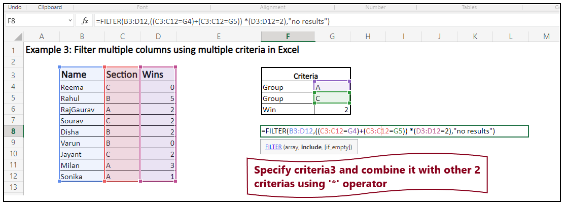
Step 4: Apply the third criteria and combine them with the rest using the ‘*’ (AND) operator.
In the third criteria, we will specify the minimum required number of wins in cell G6 (criteria3). Again, we will check if the values in between D3: D12 are equal to 2. Later combine criteria 3 with the other two using AND operator, and we will use the logical expression for AND, i.e., ‘*’.The formula will be as follows:
=FILTER(B3:D12,((C3:C12=G4)+(C3:C12=G5)) *(D3:D12=2),”no results”)
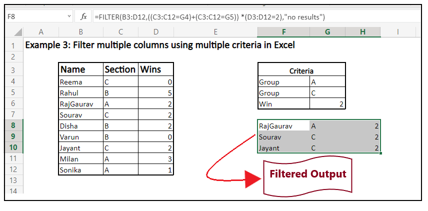
Step 5: Press the enter button to fetch the output
Excel will filter the entries based on the specified criteria and will fetch the output for you.
It will look similar to the below image:
The FILTER function not working in Excel
Many times while working with the Excel FILTER formula, there are chances you may encounter one of the following errors. Let’s see why the errors occur and how to fix them:
#CALC! error
This error occurs if you have dropped the optional if_empty argument and the function is not able to fetch any output because none of the values met the criteria. The primary reason for this error is because the Excel worksheets do not support empty arrays.
To fix the #CALC! error, make sure to always specify a value in the optional if_empty argument while defining the Excel FILTER function.
#VALUE error
You may have to deal with this error if you have entered incompatible dimensions in the array and include arguments.
To prevent such errors, always make sure to enter valid values in the FILTER arguments.
#N/A, #VALUE, etc.
You may encounter with these typed Different errors while working with FILTER function. The main reason these errors may occur if you have entered invalid value in the include argument that cannot be converted to a Boolean (TRUE or FALSE).
Always remember to include a criteria in the include argument that can be converted to Boolean value.
#NAME error
The #NAME error occurs when you implement the FILTER function in the older version that don’t support it. Always make sure to use this function only in the latest Excel versions i.e., Office 365 and Excel 2021.
You make also encounter this error in the new Excel versions, if mistakenly you have misspelt the function’s name.
#SPILL error
This error may occur if one or more cells in the spill range have some values and are not empty.
To prevent this error, you only need to clear or delete the data from the spill range.
#REF! error
The #REF! error occurs when you use the FILTER function in between different workbooks, and the primary workbook is closed.
Congratulations! Now you have briefly understood about the FILTER function. Go ahead and filter your data using the Excel Filter function.