R Built-in Functions
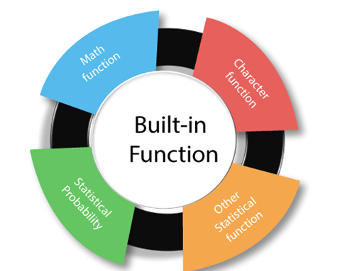
The functions which are already created or defined in the programming framework are known as a built-in function. R has a rich set of functions that can be used to perform almost every task for the user. These built-in functions are divided into the following categories based on their functionality.
Math Functions
R provides the various mathematical functions to perform the mathematical calculation. These mathematical functions are very helpful to find absolute value, square value and much more calculations. In R, there are the following functions which are used:
| S. No | Function | Description | Example |
|---|---|---|---|
| 1. | abs(x) | It returns the absolute value of input x. | x<- -4 print(abs(x)) Output [1] 4 |
| 2. | sqrt(x) | It returns the square root of input x. | x<- 4 print(sqrt(x)) Output [1] 2 |
| 3. | ceiling(x) | It returns the smallest integer which is larger than or equal to x. | x<- 4.5 print(ceiling(x)) Output [1] 5 |
| 4. | floor(x) | It returns the largest integer, which is smaller than or equal to x. | x<- 2.5 print(floor(x)) Output [1] 2 |
| 5. | trunc(x) | It returns the truncate value of input x. | x<- c(1.2,2.5,8.1) print(trunc(x)) Output [1] 1 2 8 |
| 6. | round(x, digits=n) | It returns round value of input x. | x<- -4 print(abs(x)) Output 4 |
| 7. | cos(x), sin(x), tan(x) | It returns cos(x), sin(x) value of input x. | x<- 4 print(cos(x)) print(sin(x)) print(tan(x)) Output [1] -06536436 [2] -0.7568025 [3] 1.157821 |
| 8. | log(x) | It returns natural logarithm of input x. | x<- 4 print(log(x)) Output [1] 1.386294 |
| 9. | log10(x) | It returns common logarithm of input x. | x<- 4 print(log10(x)) Output [1] 0.60206 |
| 10. | exp(x) | It returns exponent. | x<- 4 print(exp(x)) Output [1] 54.59815 |
String Function
R provides various string functions to perform tasks. These string functions allow us to extract sub string from string, search pattern etc. There are the following string functions in R:
| S. No | Function | Description | Example |
|---|---|---|---|
| 1. | substr(x, start=n1,stop=n2) | It is used to extract substrings in a character vector. | a <- "987654321" substr(a, 3, 3) Output [1] "3" |
| 2. | grep(pattern, x , ignore.case=FALSE, fixed=FALSE) | It searches for pattern in x. | st1 <- c('abcd','bdcd','abcdabcd') pattern<- '^abc' print(grep(pattern, st1)) Output [1] 1 3 |
| 3. | sub(pattern, replacement, x, ignore.case =FALSE, fixed=FALSE) | It finds pattern in x and replaces it with replacement (new) text. | st1<- "England is beautiful but no the part of EU" sub("England', "UK", st1) Output [1] "UK is beautiful but not a part of EU" |
| 4. | paste(…, sep=””) | It concatenates strings after using sep string to separate them. | paste('one',2,'three',4,'five') Output [1] one 2 three 4 five |
| 5. | strsplit(x, split) | It splits the elements of character vector x at split point. | a<-"Split all the character" print(strsplit(a, "")) Output [[1]] [1] "split" "all" "the" "character" |
| 6. | tolower(x) | It is used to convert the string into lower case. | st1<- "shuBHAm" print(tolower(st1)) Output [1] shubham |
| 7. | toupper(x) | It is used to convert the string into upper case. | st1<- "shuBHAm" print(toupper(st1)) Output [1] SHUBHAM |
Statistical Probability Functions
R provides various statistical probability functions to perform statistical task. These statistical functions are very helpful to find normal density, normal quantile and many more calculation. In R, there are following functions which are used:
| S. No | Function | Description | Example |
|---|---|---|---|
| 1. | dnorm(x, m=0, sd=1, log=False) | It is used to find the height of the probability distribution at each point to a given mean and standard deviation | a <- seq(-7, 7, by=0.1) b <- dnorm(a, mean=2.5, sd=0.5) png(file="dnorm.png") plot(x,y) dev.off() |
| 2. | pnorm(q, m=0, sd=1, lower.tail=TRUE, log.p=FALSE) | it is used to find the probability of a normally distributed random numbers which are less than the value of a given number. | a <- seq(-7, 7, by=0.2) b <- dnorm(a, mean=2.5, sd=2) png(file="pnorm.png") plot(x,y) dev.off() |
| 3. | qnorm(p, m=0, sd=1) | It is used to find a number whose cumulative value matches with the probability value. | a <- seq(1, 2, by=002) b <- qnorm(a, mean=2.5, sd=0.5) png(file="qnorm.png") plot(x,y) dev.off() |
| 4. | rnorm(n, m=0, sd=1) | It is used to generate random numbers whose distribution is normal. | y <- rnorm(40) png(file="rnorm.png") hist(y, main="Normal Distribution") dev.off() |
| 5. | dbinom(x, size, prob) | It is used to find the probability density distribution at each point. | a<-seq(0, 40, by=1) b<- dbinom(a, 40, 0.5) png(file="pnorm.png") plot(x,y) dev.off() |
| 6. | pbinom(q, size, prob) | It is used to find the cumulative probability (a single value representing the probability) of an event. | a <- pbinom(25, 40,0.5) print(a) Output [1] 0.9596548 |
| 7. | qbinom(p, size, prob) | It is used to find a number whose cumulative value matches the probability value. | a <- qbinom(0.25, 40,01/2) print(a) Output [1] 18 |
| 8. | rbinom(n, size, prob) | It is used to generate required number of random values of a given probability from a given sample. | a <- rbinom(6, 140,0.4) print(a) Output [1] 55 61 46 56 58 49 |
| 9. | dpois(x, lamba) | it is the probability of x successes in a period when the expected number of events is lambda (λ) | dpois(a=2, lambda=3)+dpois(a=3, lambda=3)+dpois(z=4, labda=4) Output [1] 0.616115 |
| 10. | ppois(q, lamba) | It is a cumulative probability of less than or equal to q successes. | ppois(q=4, lambda=3, lower.tail=TRUE)-ppois(q=1, lambda=3, lower.tail=TRUE) Output [1] 0.6434504 |
| 11. | rpois(n, lamba) | It is used to generate random numbers from the poisson distribution. | rpois(10, 10) [1] 6 10 11 3 10 7 7 8 14 12 |
| 12. | dunif(x, min=0, max=1) | This function provide information about the uniform distribution on the interval from min to max. It gives the density. | dunif(x, min=0, max=1, log=FALSE) |
| 13. | punif(q, min=0, max=1) | It gives the distributed function | punif(q, min=0, max=1, lower.tail=TRUE, log.p=FALSE) |
| 14. | qunif(p, min=0, max=1) | It gives the quantile function. | qunif(p, min=0, max=1, lower.tail=TRUE, log.p=FALSE) |
| 15. | runif(x, min=0, max=1) | It generates random deviates. | runif(x, min=0, max=1) |
Other Statistical Function
Apart from the functions mentioned above, there are some other useful functions which helps for statistical purpose. There are the following functions:
| S. No | Function | Description | Example |
|---|---|---|---|
| 1. | mean(x, trim=0, na.rm=FALSE) | It is used to find the mean for x object | a<-c(0:10, 40) xm<-mean(a) print(xm) Output [1] 7.916667 |
| 2. | sd(x) | It returns standard deviation of an object. | a<-c(0:10, 40) xm<-sd(a) print(xm) Output [1] 10.58694 |
| 3. | median(x) | It returns median. | a<-c(0:10, 40) xm<-meadian(a) print(xm) Output [1] 5.5 |
| 4. | quantilie(x, probs) | It returns quantile where x is the numeric vector whose quantiles are desired and probs is a numeric vector with probabilities in [0, 1] | |
| 5. | range(x) | It returns range. | a<-c(0:10, 40) xm<-range(a) print(xm) Output [1] 0 40 |
| 6. | sum(x) | It returns sum. | a<-c(0:10, 40) xm<-sum(a) print(xm) Output [1] 95 |
| 7. | diff(x, lag=1) | It returns differences with lag indicating which lag to use. | a<-c(0:10, 40) xm<-diff(a) print(xm) Output [1] 1 1 1 1 1 1 1 1 1 1 30 |
| 8. | min(x) | It returns minimum value. | a<-c(0:10, 40) xm<-min(a) print(xm) Output [1] 0 |
| 9. | max(x) | It returns maximum value | a<-c(0:10, 40) xm<-max(a) print(xm) Output [1] 40 |
| 10. | scale(x, center=TRUE, scale=TRUE) | Column center or standardize a matrix. | a <- matrix(1:9,3,3) scale(x) Output [,1] [1,] -0.747776547 [2,] -0.653320562 [3,] -0.558864577 [4,] -0.464408592 [5,] -0.369952608 [6,] -0.275496623 [7,] -0.181040638 [8,] -0.086584653 [9,] 0.007871332 [10,] 0.102327317 [11,] 0.196783302 [12,] 3.030462849 attr(,"scaled:center") [1] 7.916667 attr(,"scaled:scale") [1] 10.58694 |