R-Random Forest

The Random Forest is also known as Decision Tree Forest. It is one of the popular decision tree-based ensemble models. The accuracy of these models is higher than other decision trees. This algorithm is used for both classification and regression applications.

In a random forest, we create a large number of decision trees, and in each decision tree, every observation is fed. The final output is the most common outcome for each observation. We take a majority vote for each classification model by feeding a new observation into all the trees.

An error estimate is made for cases that were not used when constructing the tree. This is called an out-of-bag(OOB) error estimate mentioned as a percentage.

The decision trees are prone to overfitting, and this is the main drawback of it. The reason is that trees, if deepened, are able to fit all types of variations in the data, including noise. It is possible to address this by partial pruning, and the results are often less than satisfactory.

R allows us to create random forests by providing the randomForest package. The randomForest package provides randomForest() function, which helps us to create and analyze random forests. There is the following syntax of random forest in R:

Example:

Let’s start understanding how the randomForest package and its function are used. For this, we take an example in which we used the heart-disease dataset. Let’s start our coding section step by step.

1) In the first step, we have to load the three required libraries i.e., ggplot2, cowplot, and randomForest.

  #Loading ggplot2, cowplot, and randomForest packages   library(ggplot2)  library(cowplot)  library(randomForest)  

2) Now, we will use the heart-disease dataset present in http://archive.ics.uci.edu/ml/machine-learning-databases/heart-disease/processed.cleveland.data. And then, from this dataset, we read the data in CSV format and store it in a variable.

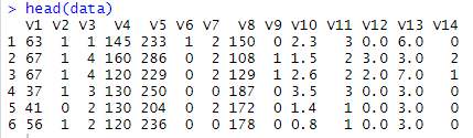
  #Fetching heart-disease dataset  url<-“http://archive.ics.uci.edu/ml/machine-learning-databases/heart-disease/processed.cleveland.data”  data <- read.csv(url,header=FALSE)  

3) Now, we print our data with the help of head() function which prints only the starting six rows as:

When we run the above code, it will generate the following output.

Output:

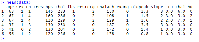
4) From the above output, it is clear that none of the columns are labeled. Now, we name the columns and make these columns labeled in the following way:

  colnames(data) <-c(“age”,”sex”,”cp”,”trestbps”,”chol”,”fbs”,”restecg”,”thalach”,”exang”,”oldpeak”,”slope”,”ca”,”thal”,”hd”)  head(data)  

Output:

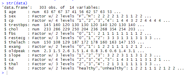
5) Let’s check the structure of the data with the help of str() function to analyze it better.

Output:

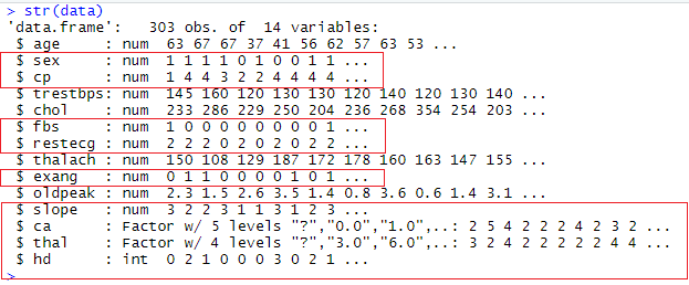
6) In the above output, we highlight those columns which we will use in our analysis. It is clear from the output that some of the columns are messed up. Sex is supposed to be a factor where 0 represents the “Female” and 1 represents the “Male”. And cp(chest pain) is also supposed to be a factor where level 1 to 3 represent a different type of pain, and 4 represent no chest pain.

The ca and thal are factors, but one of the levels is “?” when we need it to be NA. We have to clean up the data in our dataset, which are as follows:

  #Changing the “?” to NAs?   data[data==”?”] <- NA    #Converting the 0’s in sex to F and 1’s to M  data[data$sex==0,]$sex <-“F”  data[data$sex==1,]$sex <-“M”    #Converting columns tnto the factors  data$sex<- as.factor(data$sex)  data$cp<- as.factor(data$cp)  data$fbs<- as.factor(data$fbs)  data$restecg<- as.factor(data$restecg)  data$exang<- as.factor(data$exang)  data$slope<- as.factor(data$slope)    #ca and thal columns contain? rather than NA. R treats it as a column of string, We correct this assumption by telling R that is a column of integers.     data$ca<- as.integer(data$ca)  data$ca<- as.factor(data$ca)  data$thal<- as.integer(data$thal)  data$thal<- as.factor(data$thal)    #Making data hd where 0’s represent healthy and 1’s to unhealthy.  data$hd<- ifelse(test=data$hd==0,yes=”healthy”,no=”Unhealthy”)  data$hd<- as.factor(data$hd)    #Checking structure of data  str(data)  

Output:

7) Now, we are randomly sampling things by setting the seed for the random number generator so that we can reproduce our result.

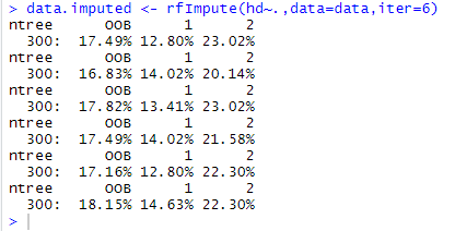
8) NWxt, we impute values for the NAs in the dataset with rfImput() function. In the following way:

Output:

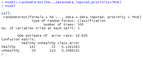
9) Now, we build the proper random forest with the help of the randomForest() function in the following way:

Output:

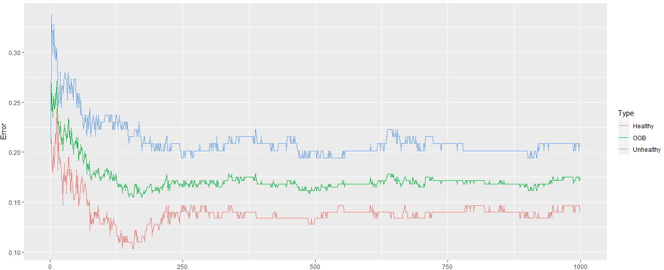
10) Now, if 500 trees are enough for optimal classification, we will plot the error rates. We create a data frame which will format the error rate information in the following way:

  oob_error_data<- data.frame(Trees=rep(1:nrow(Model$err.rate),times=3),Type=rep(c(“OOB”,”Healthy”,”Unhealthy”),each=nrow(Model$err.rate)),Error=c(Model$err.rate[,”OOB”],Model$err.rate[,”healthy”],Model$err.rate[,”Unhealthy”]))  

11) We call the ggplot for plotting error rate in the following way:

  11) We call the ggplot for plotting error rate in the following way:  ggplot(data=oob_error_data,aes(x=Trees,y=Error))+geom_line(aes(color=Type))  

Output:

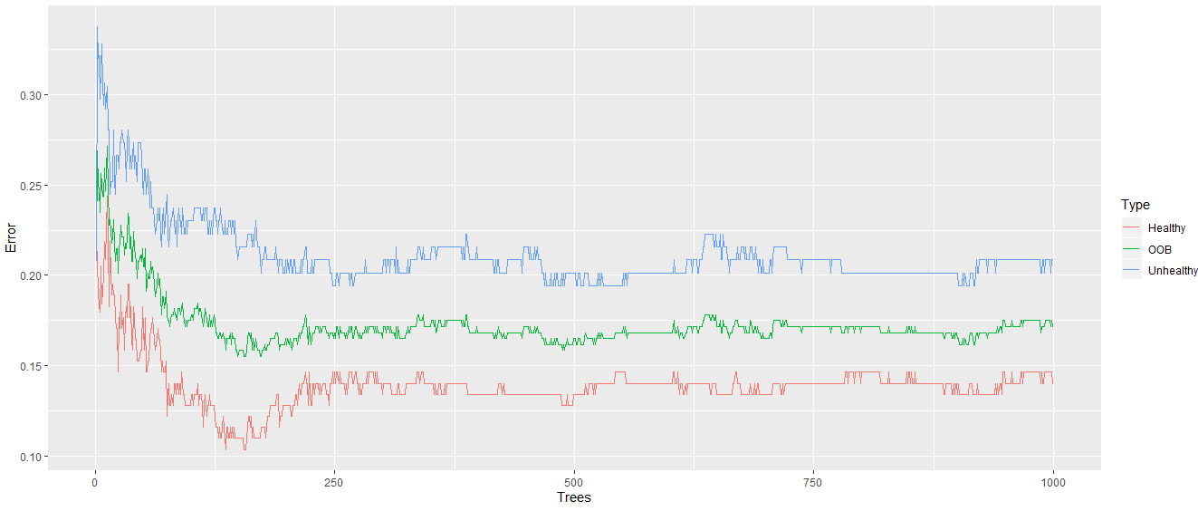
From the above output, it is clear that the error rate decreases when our random forest has more trees.

12) Now, we add 1000 trees and check would the error rate goes down further? So we make a random forest with 1000 trees and find the error rate as we have done before.

Output:

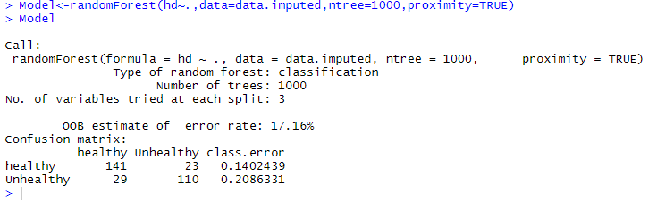
  oob_error_data<- data.frame(Trees=rep(1:nrow(Model$err.rate),times=3),Type=rep(c(“OOB”,”Healthy”,”Unhealthy”),each=nrow(Model$err.rate)),Error=c(Model$err.rate[,”OOB”],Model$err.rate[,”healthy”],Model$err.rate[,”Unhealthy”]))  ggplot(data=oob_error_data,aes(x=Trees,y=Error))+geom_line(aes(color=Type))  

Output:

From the above output it is clear that the error rate is stabilized.

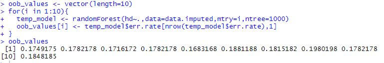
13) Now, we need to make sure that we are considering the optimal number of variables at each internal node in the tree. This will be done in the following way:

  #Creating a vector that can hold ten values.  oob_values<- vector(length=10)    #Testing of the different numbers of variables at each step.  for(i in 1:10){    #Building a random forest for determining the number of variables to try at each step.  temp_model<- randomForest(hd~.,data=data.imputed,mtry=i,ntree=1000)      #Storing OOB error rate.  oob_values[i] <- temp_model$err.rate[nrow(temp_model$err.rate),1]  }  oob_values  

Output:

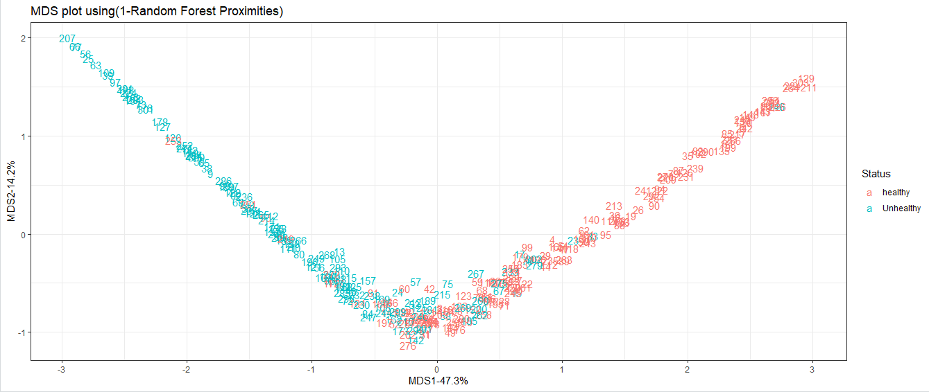
14) Now, we use the random forest to draw an MDS plot with samples. This will show us how they are related to each other. This will be done in the following way:

  #Creating a distance matrix with the help of dist() function.  distance_matrix<- dist(1-Model$proximity)    #Running cmdscale() on the distance matrix.   mds_stuff<- cmdscale(distance_matrix,eig=TRUE,x.ret=TRUE)    #Calculating the percentage of variation in the distance matrix that the X and Y axes account for.  mds_var_per<- round(mds_stuff$eig/sum(mds_stuff$eig)*100,1)    #Formatting the data for ggplot() function  mds_values<- mds_stuff$points  mds_data<- data.frame(Sample=rownames(mds_values),X=mds_values[,1],Y=mds_values[,2],Status=data.imputed$hd)    #Drawing the graph with ggplot() function.  ggplot(data=mds_data,aes(x=X,y=Y,label=Sample))+geom_text(aes(color=Status))+theme_bw()+xlab(paste(“MDS1-“,mds_var_per[1],”%”,sep=””))+ylab(paste(“MDS2-“,mds_var_per[2],”%”,sep=””))+ggtitle(“MDS plot using(1-Random Forest Proximities)”)  

Output:

Next TopicT-Test in R

R Random Forest

R-Random Forest

Example:

Some Cryptocurrency Libraries for Python

Download and Installation of SoapUI

You may also like