SciPy Optimize

The optimize package provides various commonly used optimization algorithms. This module contains the following aspects:

Global optimization routines(brute-force, anneal(), basinhopping())
Unconstrained and constrained minimization of the multivariate scalar functions(minimize()) using various algorithms (BFGS, Nelders-Mead simplex, Newton Conjugate Gradient, COBLYA).
Least-squares minimization algorithms(leastsq() and curve fit())
Scalar univariate function minimizers (minimizer_scalar() and root finders newton())

Nelder- Mead Simplex Algorithm

The Nelder- Mead Simplex algorithm provides minimize() function which is used for minimization of scalar function of one or more variables.

  import numpy as np  import scipy  from scipy.optimize import minimize  #define function f(x)  def f(x):         return .2*(1 – x[0])**2  scipy.optimize.minimize(f, [2, -1], method=”Nelder-Mead”)  

Output:

final_simplex: (array([[ 1.        , -1.27109375],         [ 1.        , -1.27118835],         [ 1.        , -1.27113762]]), array([0., 0., 0.]))             fun: 0.0         message: 'Optimization terminated successfully.'            nfev: 147             nit: 69          status: 0         success: True               x: array([ 1.        , -1.27109375])

Least Square Minimization

It is used to solve the nonlinear least-square problems with bound on the variables. Given the residuals (difference between observed and predicted value of data) f(x) (an n-dimension real function of n real variables) and the loss function rho(s) (a scalar function), least_square finds a local minimum of the cost function f(x): Let’s consider the following example:

  from scipy.optimize import least_squares  import numpy as np  input = np.array([2, 2])  def rosenbrock(x):     return np.array([10 * (x[1] – x[0]**3), (1 – x[0])])  res = least_squares(rosenbrock, input)  print(res)  

Output:

active_mask: array([0., 0.])          cost: 0.0           fun: array([0., 0.])          grad: array([0., 0.])           jac: array([[-30.00000045,  10.        ],         [ -1.        ,   0.        ]])       message: '`gtol` termination condition is satisfied.'          nfev: 4          njev: 4    optimality: 0.0        status: 1       success: True             x: array([1., 1.])

Root Finding

Scalar functions

There are four different root-finding algorithms for a single value equation. Each algorithm needs the endpoints of an interval in which a root is expected (because the function changes signs).

Sets of Equations

The root() function is used to find the root of the nonlinear equation. There are various methods such as hybr (the default) and the Levenberg-Marquardt method from the MINPACK.

Let’s consider the below equation

x² + 3cos(x)=0

  import numpy as np  from scipy.optimize import root  def func(x):     return x*2 +  3* np.cos(x)  a = root(func, 0.3)  print(a)  

Output:

fjac: array([[-1.]])    fun: array([2.22044605e-16])   message: 'The solution converged.'      nfev: 10       qtf: array([-1.19788401e-10])         r: array([-4.37742564])    status: 1   success: True         x: array([-0.91485648])

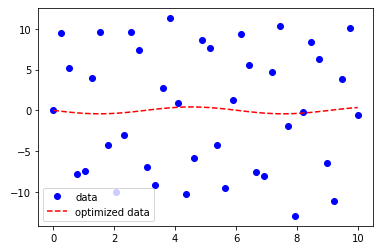
Optimize Curve Fitting

Curve fitting is the technique of creating a curve. It is a mathematical function that has the best fit to a series of data points, possibly subject to constraints. The example is given below:

  import numpy as np   from scipy.optimize import curve_fit   from matplotlib import pyplot as plt   x = np.linspace(0, 10, num = 40)   # The coefficients are much bigger.   y = 10.35 * np.sin(5.330 * x) + np.random.normal(size = 40)   def test(x, a, b):   return a * np.sin(b * x)   param, param_cov = curve_fit(test, x, y)   print(“Sine funcion coefficients:”)   print(param)   print(“Covariance of coefficients:”)   print(param_cov)   ans = (param[0]*(np.sin(param[1]*x)))   plt.plot(x, y, ‘o’, color =’red’, label =”data”)   plt.plot(x, ans, ‘–‘, color =’blue’, label =”optimized data”)   plt.legend()   plt.show()  

Output:

Sine funcion coefficients:  [-0.42111847  1.03945217]  Covariance of coefficients:  [[3.03920718 0.05918002]   [0.05918002 0.43566354]]

SciPy fsolve

The scipy.optimize library provides the fsolve() function, which is used to find the root of the function. It returns the roots of the equation defined by fun(x) = 0 given a starting estimate.

Consider the following example:

  import numpy as np  from scipy.optimize import fsolve  sqrt = np.emath.sqrt  a = 132712000000  T = 365.35 * 86337 * 2 / 3  e = 580.2392124070273  def f(x):      return np.abs((T * a ** 2 / (2 * np.pi)) ** (1 / 3) * sqrt(1 – x ** 2)          – sqrt(.5 * a ** 2 / e * (1 – x ** 2)))  x = fsolve(f, 0.01)  x, f(x)  

Output:

(array([1.]), array([82.17252895]))

Next TopicSciPy Stats

SciPy Optimize

SciPy Optimize

Nelder- Mead Simplex Algorithm

Least Square Minimization

Root Finding

Optimize Curve Fitting

SciPy fsolve

Singleton Design Pattern in Python

Data Visualization in Python using Bokeh Library

You may also like