Sequence Function in Excel
Sequencing your data in an Excel worksheet is a tedious task. But fortunately, those days are long gone! Though many users may think of using the AutoFill feature to list down the numbers series in a sequence. But this modern autofill feature doesn’t work if you have a more specified sequential task to perform. Therefore, in such cases, you can use the inbuilt SEQUENCE function, which is specially created for this pursuit.
In this tutorial, you will learn what is Sequence function, its syntax, parameter, points to remember, how this formula works and various examples by using the Sequence function to return a new dynamic array by auto-generating a series of Roman numbers and random integers
What is Sequence Function?
“The SEQUENCE function is an inbuilt Excel function that generates an array of sequential numbers whether number, roman number, alphabets. For example: 1, 2, 3, etc.“
The SEQUENCE function is a new dynamic array function that generates a list of sequential numbers in an array. Though the resultant array can be one-dimensional or two-dimensional, determined by the specified parameters i.e., rows and columns. This function always returns a dynamic array that arranging the rows and columns in the specified sequence.
The SEQUENCE function is introduced in the new Microsoft Excel 365. Therefore, if you are using the previous Excel versions, this function won’t be available. To use this function, make sure to update your Excel version to Excel 365 or above.
NOTE: If you are trying to access the Sequence function in previous Excel versions, unlike Excel 2019, Excel 2016, and lower, you won’t find it.
Syntax
Parameters
Rows (required) – This parameter represents the number of rows to sequence your data.
Columns (optional) – This parameter represents the number of columns to fill. If the user doesn’t provide this argument, by default it takes 1.
Start (optional) – This parameter represents the starting number in the sequence. If the user doesn’t provide this argument, by default it takes 1.
Step (optional) – This parameter represents the increment or decrement for each subsequent value in the sequence. It can take the following values:
- If you provide a positive number, the start number gets added in the subsequent value, producing an ascending sequential order.
- If you provide a negative number, the start number gets subtracted from the subsequent values decrease, creating a sequential order.
- If you don’t provide any value to this parameter, by default it takes 1.
Return Type
The Excel Sequence Function returns a dynamic array by automatically arranging the rows and columns in the specified sequence.
Formula to create a number sequence in Excel
If you want to create a column of rows with sequential numbers starting at 1, you can use the Excel SEQUENCE function in its simplest form:
To place values in the first row:
=SEQUENCE(1)
To put value in a column:
SEQUENCE(1, n)
Where n represents the number of values available in the sequence.
For instance, to create a column with 100 numbers, enter the following formula in the first cell (we have takes B2 in our case) and press the Enter button:
=SEQUENCE(100)
The output will be automatically be spilled in the rows starting from the selected row.
Things to Remember about Sequence Function
Before working on Microsoft Excel Sequence Function, make sure to go through with the below facts:
- The SEQUENCE function is only available in the Microsoft Excel 365 or the newer versions. Therefore, if you are using the previous Excel versions (2019, 2018, etc), this function won’t be available and it won’t create dynamic arrays.
- If the array of sequential numbers is the final output, Excel aligns all the numbers automatically in a spill range. So, always make sure you provide sufficient empty cells (using the rows and columns parameter) to the down and right of the cell where you enter the formula; otherwise, Excel will throw a #SPILL error.
- The returned array can be 1-dimensional or 2-dimensional depending upon how you pass the rows and parameters in the Sequence function.
- If any optional parameter is omitted, by default, its value is 1.
Examples:
#SEQUENCE Example1: How to create a number sequence in descending order in Excel
In the below sheet, as you see we have a list of values organised in a random order.
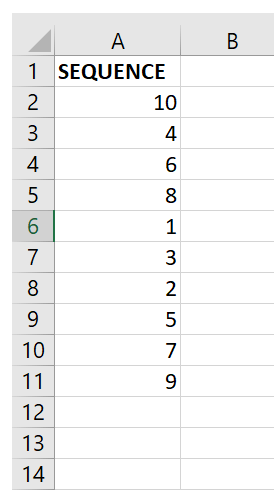
As asked in the question, to arrange the values in their descending order using the Sequence function, we just need to do a little trick, i.e., we will supply negative one (-1) in the step parameter.
Follow the below-given steps to fetch the descending sequential series of the above-given numbers using the Excel Sequence() function:
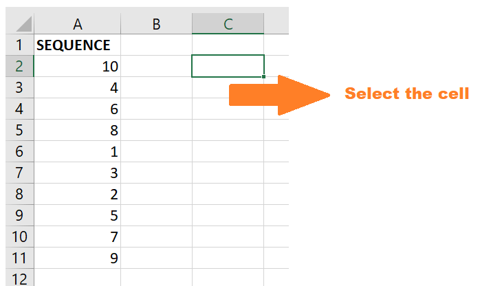
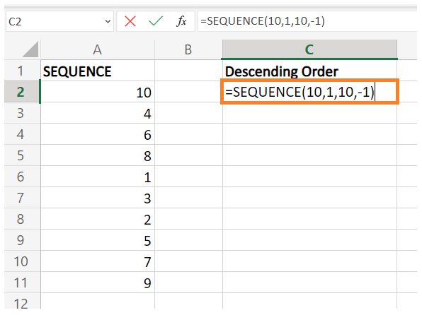
Step 1: Select a cell to position your Sequenced data
Place your mouse cursor to a cell from where you want to start the sequencing of your data. In our case, we have selected cell C2 of our Excel worksheet.
Refer to the given below image:
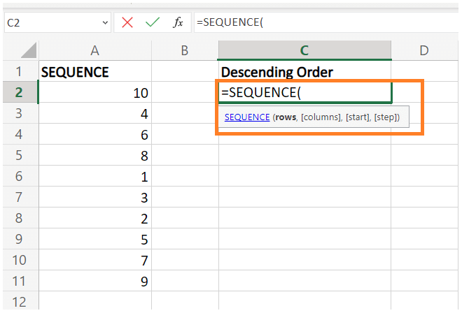
STEP 2: Type the SEQUENCE function
In the selected cell, we will start your function with the equal to (=) sign followed by the Sequence function. The formula will be as follows: = SEQUENCE(
STEP 3: Insert all the parameters
- At first, this function will ask you to specify the ROWS parameter. We will specify the number to fill and sequence the values. Since we have 10 values so here we will mention 10. The formula will be = SEQUENCE(10,
- The next argument is Column. This parameter represents the Column to start the sequence here we will specify 1. = SEQUENCE(10,1,
- Next, specify the start parameter. In this, we will specify the value we want to start our sequencing with. Here we will mention 10. = SEQUENCE(10,1,10
- Since we want the sequencing to be ordered in descending order. Therefore in the step parameter, we will specify -1. = SEQUENCE(10,1,10,-1)
Step 4: The Sequence function will return the output
As a result, the SEQUENCE function will return the 10 numbers in descending sequential order.
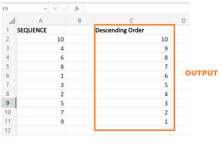
Explanation
This function will select 10 values and start the counting from 10. It will subtract 1 from 10, and return 9. Again, it will subtract 1 and return 8, and in the pattern, it will return 10 values in the descending sequential order.
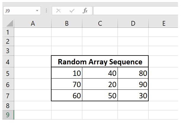
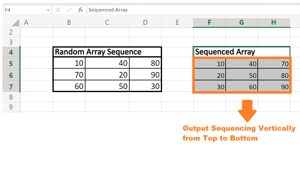
#SEQUENCE Example2: How to create a 2-D array where sequential order moves vertically top to bottom.
When working with an array of cells, the standard sequencing rule goes horizontally across the first row till its last element, and next, it moves down to the next row, in a similar method to reading text from left to right. But in various scenarios, the range of cells is not listed in sequential order as per the given Excel data.
To propagate the above data in the top to bottom order across the first column and then right to the next column, we will use the combination of the SEQUENCE function and the TRANSPOSE function. Follow the below-given steps to fetch the results using Excel SEQUENCE() function:
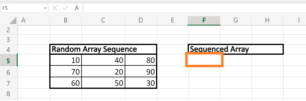
Step 1: Select a cell to position your Sequenced data
Place your mouse cursor to a cell from where you want to start the sequencing of your data. In our case, we have selected cell F2 of our Excel worksheet.
Refer to the given below image:
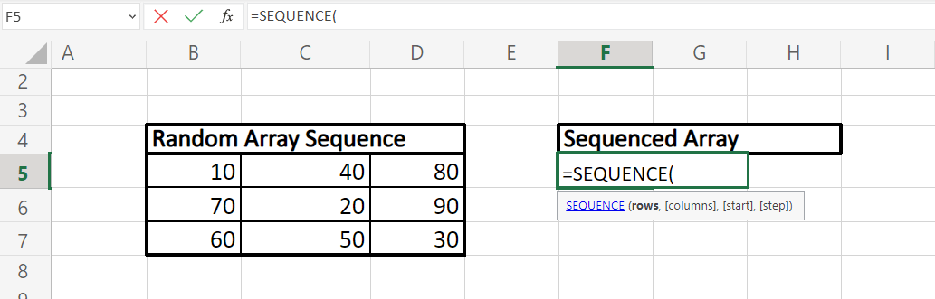
STEP 2: Type the SEQUENCE function
In the selected cell, we will start your function with the equal to (=) sign followed by the Sequence function. The formula will be as follows: = SEQUENCE(
STEP 3: Insert all the parameters
- At first, this function will ask you to specify the ROWS parameter. Since in our case we have our data in three rows. Therefore, we will specify 3 in this parameter. The formula will be = SEQUENCE(3,
- The next argument is Column. This parameter represents the Column to start the sequence. Since we have 3 columns, therefore will specify 3. The formula will be = SEQUENCE(3,3,
- Next, specify the start parameter. In this, we will specify the value we want to start our sequencing with. Here we will mention 10. The formula will be = SEQUENCE(3,3,10
- Since we want the sequencing to be ordered with a gap of 10 order. Therefore, in the step parameter, we will specify 10. = SEQUENCE(3,3,10,10)
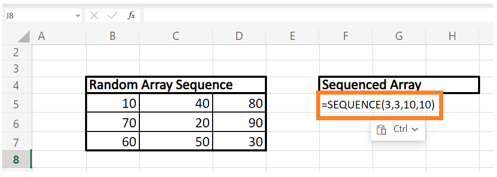
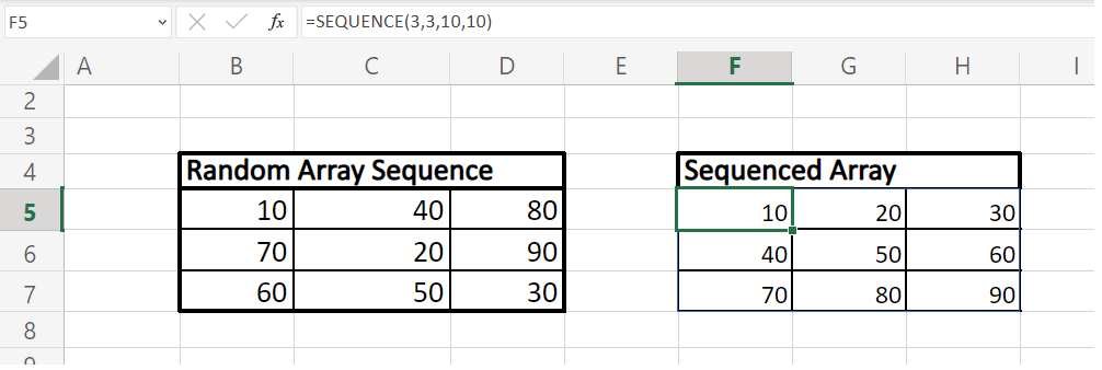
Step 4: The Sequence function will return the output
As a result, the regular SEQUENCE function will moves horizontally left to right (column-wise) and return the following maintaining a gap of 10 between the values.
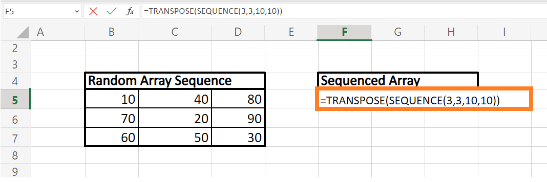
Step 5: Nest Sequence function inside the Transpose Function
Though the above output is also correct, that’s not what we were looking for. In the question, we are asked to create a sequence that moves vertically from top to bottom (row-wise), maintaining order of 10. Therefore, we will use the Transpose function and nest the above Sequence function inside it.
The formula will be as follows:
=TRANSPOSE(SEQUENCE(3, 3, 10, 10))
Step 6: Excel will fetch you the result
Once done, press the enter button and Excel will arrange all the data in the specified sequence where the is arranged in the array sequencing vertically from top to bottom (row-wise).
Refer to the below image for your reference.
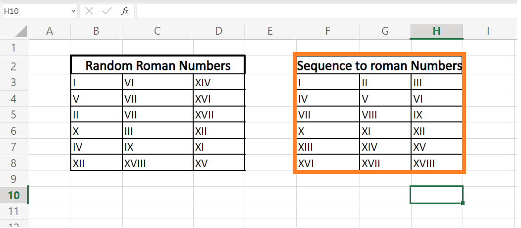
#SEQUENCE Example3: How to create a sequence of Roman numbers in Excel worksheet?
Roman numbers are an interesting method to list down your data in Excel. But have you ever tried to create a SEQUENCE formula for Roman numbers? If the answer is no! what are you waiting for?
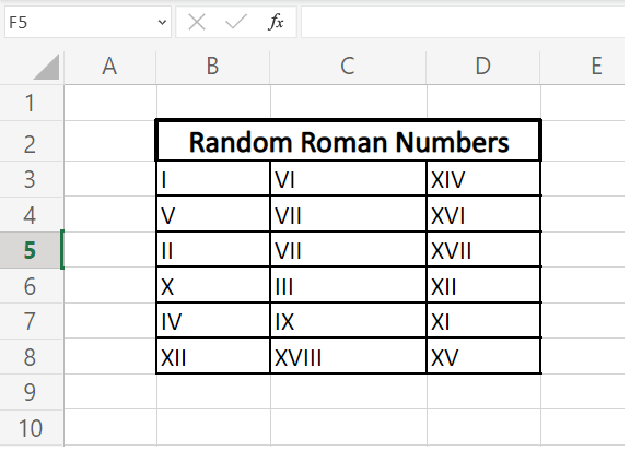
Using the inbuilt Sequence function, try to list down the roman numbers in a specified order. Give it a try; else you can take the hint from the given below steps to wrap the roman numerals in sequential order:
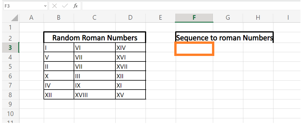
Step 1: Select a cell to position your Sequenced data
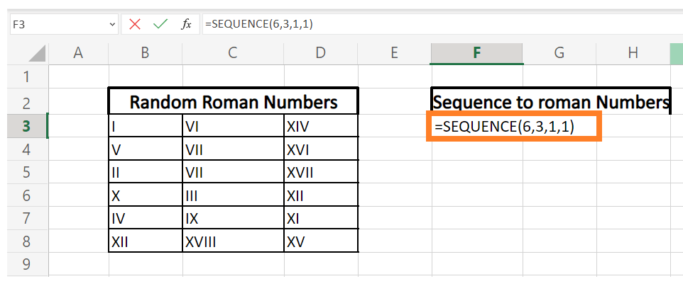
Place your mouse cursor to a cell from where you want to start the sequencing of your data. In our case, we have selected cell F3 of our Excel worksheet.
Refer to the given below image:
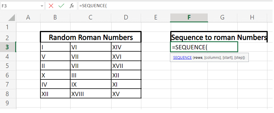
STEP 2: Type the SEQUENCE function
In the selected cell, we will start your function with the equal to (=) sign followed by the Sequence function. The formula will be as follows: = SEQUENCE(
STEP 3: Insert all the parameters
- Since we have 6 rows in our Excel listing array table, so we will specify 6 in the first parameter. The formula will be = SEQUENCE(6,
- The next argument is Column. In this parameter we will specify 3. The formula will be = SEQUENCE(6,3,
- Next, specify the start parameter. Though the data table is in roman numbers but in that also we are starting with 1. The formula will be. = SEQUENCE(6,3,1
- Since we want the sequencing to be ordered in ascending order. Therefore we will place positive 1 in this argument. The formula will be = SEQUENCE(6,3,1,1)
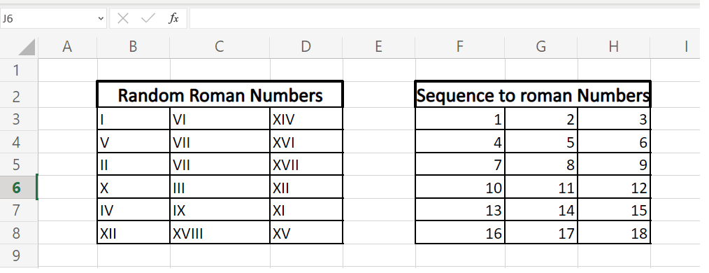
Step 4: The Sequence function will return the output
As a result, the SEQUENCE function will return the numbers arrange in ascending sequential order.
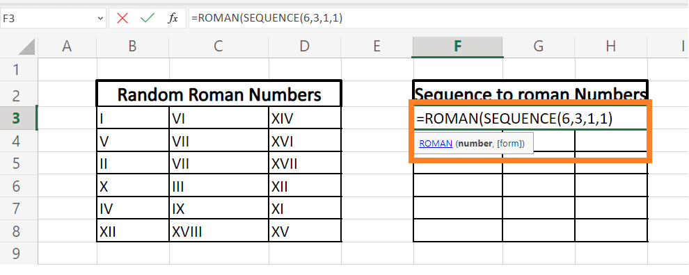
STEP 5: Nest Sequence function inside the inbuilt Excel Roman Function
In the above output, the sequence is correct, but the values are in numbers, whereas we want them to be sequenced in Roman numbers. Therefore, we will convert the sequenced numbers to roman numbers using Excel’s inbuilt Roman function.
The formula will be as follows:
=ROMAN(SEQUENCE(6, 3, 1, 1))
Step 6: Roman numbers will be sequenced
Roman numbers will be sequenced horizontally (left to right) as an output.
Refer to the below given image: