The AVERAGEIFS function in Google Sheets can be used to find the average value in a range if the corresponding values in another range meet certain criteria.
This function uses the following basic syntax:
AVERAGEIFS(average_range, criteria_range1, criterion1, [criteria_range2, criterion2, …])
where:
- average_range: The range to calculate average from
- criteria_range1: The first range to check for certain criteria
- criterion1: The criteria to analyze in the first range
The following examples show how to use this function in different scenarios with the following dataset in Google Sheets:

Example 1: AVERAGEIFS with One Character Column
We can use the following formula to calculate the average value in the Points column where the Team column is equal to “Mavs”:
=AVERAGEIFS(C2:C11, A2:A11, "Mavs")
The following screenshot shows how to use this formula in practice:

The average value in the Points column where the Team column is equal to “Mavs” is 24.6.
We can manually verify this is correct by calculating the average points for the Mavs players:
Average: (22 + 28 + 25 + 30 + 18) / 5 = 24.6.
Example 2: AVERAGEIFS with Two Character Columns
We can use the following formula to calculate the average value in the Points column where the Team column is equal to “Mavs” and the Position column is equal to “Guard”:
=AVERAGEIFS(C2:C11, A2:A11, "Mavs", B2:B11, "Guard")
The following screenshot shows how to use this formula in practice:
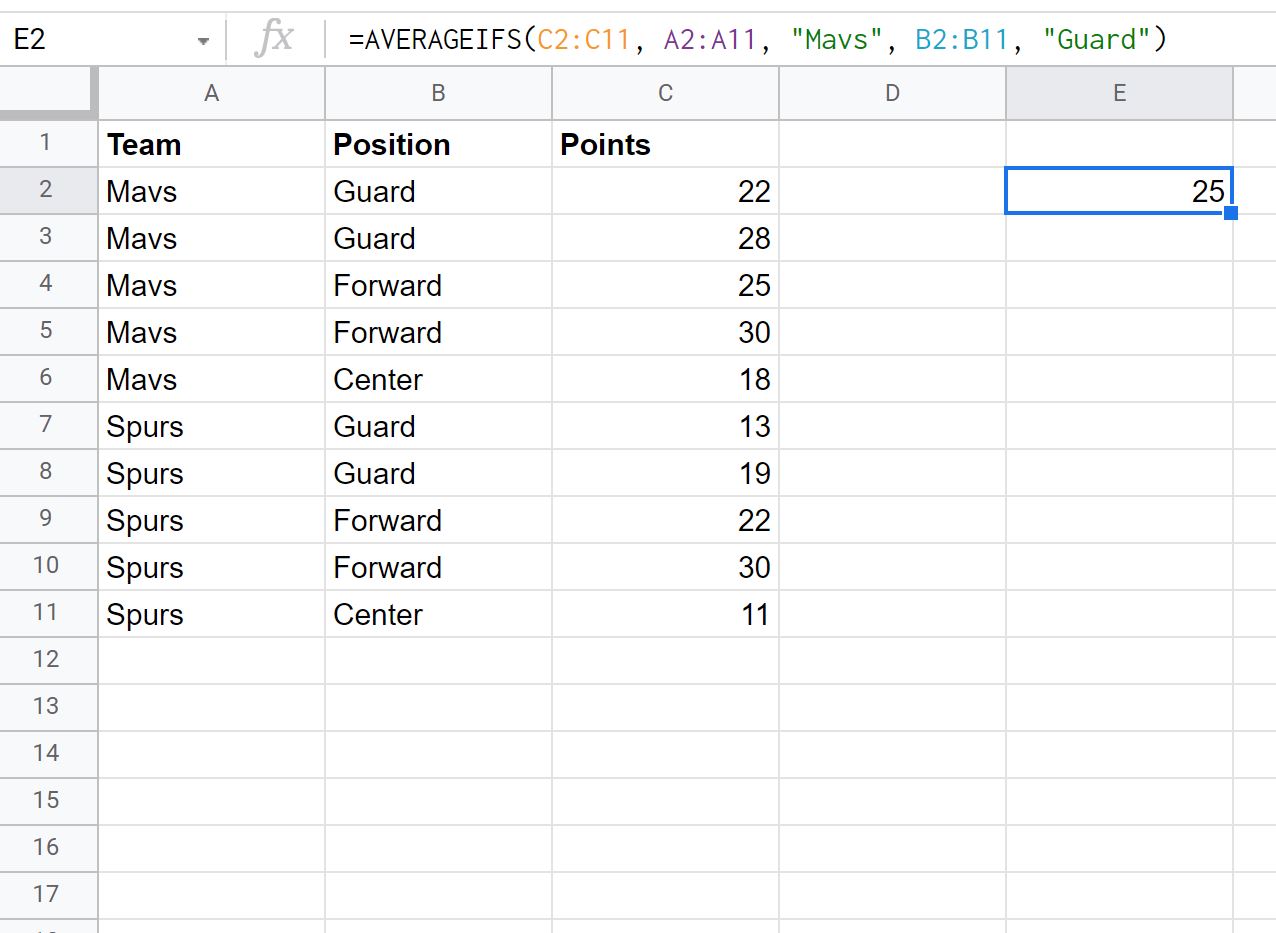
The average value in the Points column where the Team column is equal to “Mavs” and the Position column is equal to “Guard” is 29.
We can manually verify this is correct by calculating the average points for the Mavs players who are Guards:
Average: (22 + 28) / 2 = 25.
Example 3: AVERAGEIFS with Character & Numeric Columns
We can use the following formula to calculate the average value in the Points column where the Team column is equal to “Spurs” and the Points column is greater than 15:
=AVERAGEIFS(C2:C11, A2:A11, "Spurs", C2:C11, ">15")
The following screenshot shows how to use this formula in practice:

The average value in the Points column where the Team column is equal to “Spurs” and the Points column is greater than 15 is 23.67.
We can manually verify this is correct by calculating the average points for the Spurs players who scored more than 15 points:
Average: (19 + 22 + 30) / 3 = 23.67.
Note: You can find the complete online documentation for the AVERAGEIFS function here.
Additional Resources
The following tutorials explain how to perform other common tasks in Google Sheets:
Google Sheets: How to Calculate Mean, Median & Mode
Google Sheets: How to Calculate Average If Not Blank
Google Sheets: How to Calculate Exponential Moving Average