One of the most common clustering algorithms used in machine learning is known as k-means clustering.
K-means clustering is a technique in which we place each observation in a dataset into one of K clusters.
The end goal is to have K clusters in which the observations within each cluster are quite similar to each other while the observations in different clusters are quite different from each other.
When performing k-means clustering, the first step is to choose a value for K – the number of clusters we’d like to place the observations in.
One of the most common ways to choose a value for K is known as the elbow method, which involves creating a plot with the number of clusters on the x-axis and the total within sum of squares on the y-axis and then identifying where an “elbow” or bend appears in the plot.
The point on the x-axis where the “elbow” occurs tells us the optimal number of clusters to use in the k-means clustering algorithm.
The following example shows how to use the elbow method in R.
Example: Using the Elbow Method in R
For this example we’ll use the USArrests dataset built into R, which contains the number of arrests per 100,000 residents in each U.S. state in 1973 for Murder, Assault, and Rape along with the percentage of the population in each state living in urban areas, UrbanPop.
The following code shows how to load the dataset, remove rows with missing values, and scale each variable in the dataset to have a mean of 0 and standard deviation of 1:
#load data
df #remove rows with missing values
df omit(df)

#scale each variable to have a mean of 0 and sd of 1
df #view first six rows of dataset
head(df)

               Murder   Assault   UrbanPop         Rape
Alabama    1.24256408 0.7828393 -0.5209066 -0.003416473
Alaska     0.50786248 1.1068225 -1.2117642  2.484202941
Arizona    0.07163341 1.4788032  0.9989801  1.042878388
Arkansas   0.23234938 0.2308680 -1.0735927 -0.184916602
California 0.27826823 1.2628144  1.7589234  2.067820292
Colorado   0.02571456 0.3988593  0.8608085  1.864967207
To find the optimal number of clusters to use in the k-means algorithm, we’ll use the fviz_nbclust() function from the factoextra package to create a plot of the number of clusters vs. the total within sum of squares:
library(cluster)
library(factoextra)

#create plot of number of clusters vs total within sum of squares
fviz_nbclust(df, kmeans, method = "wss")
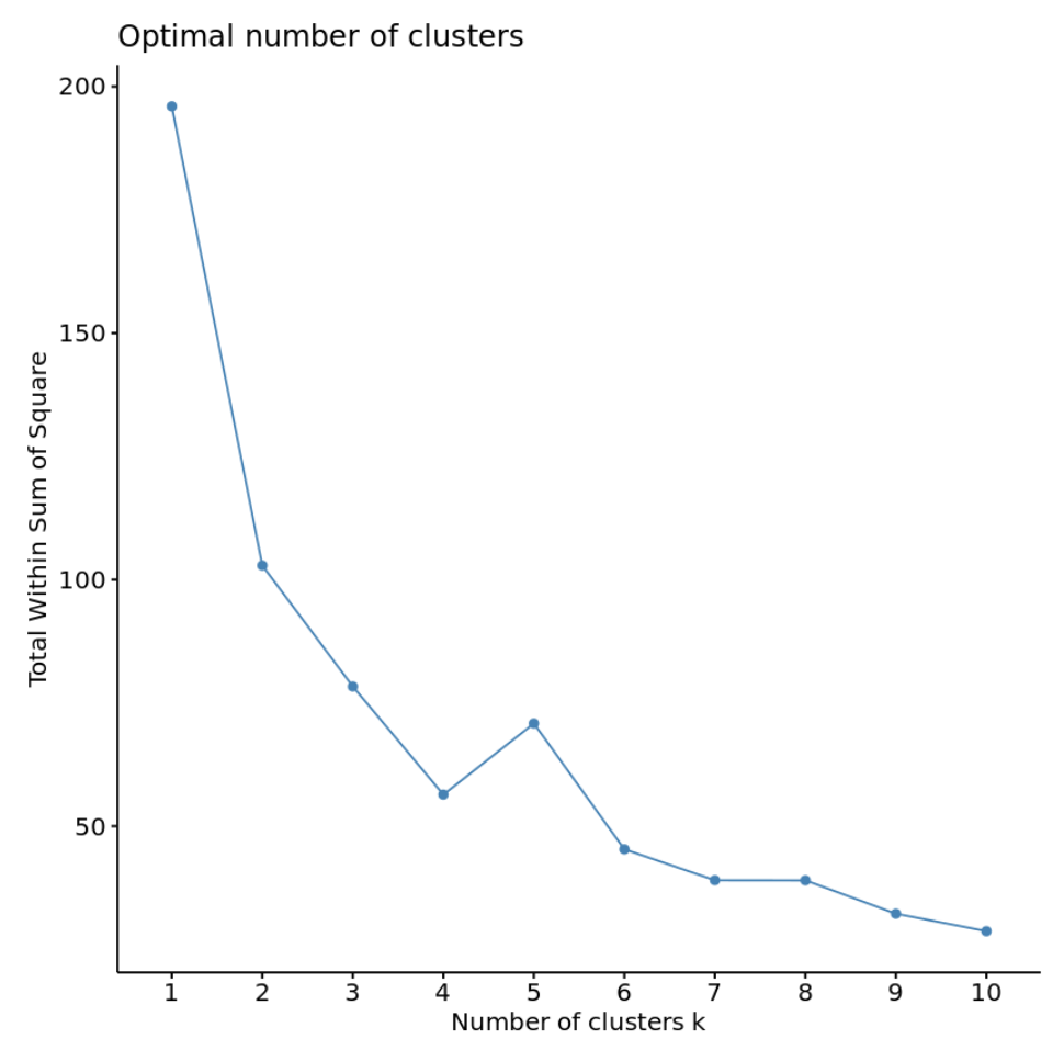
In this plot it appears that there is an “elbow” or bend at k = 4 clusters. This is the point where the total within sum of squares begins to level off.
This tells us that the optimal number of clusters to use in the k-means algorithm is 4.
Note: Although we could achieve a lower total within sum of squares by using more clusters, we would likely be overfitting the training data and thus the k-means algorithm wouldn’t perform as well on testing data.
We can proceed to use the kmeans() function from the cluster package to perform k-means clustering on the dataset using the optimal value for k of 4:
#make this example reproducible
set.seed(1)

#perform k-means clustering with k = 4 clusters
km #view results
km

K-means clustering with 4 clusters of sizes 16, 13, 13, 8

Cluster means:
      Murder    Assault   UrbanPop        Rape
1 -0.4894375 -0.3826001  0.5758298 -0.26165379
2 -0.9615407 -1.1066010 -0.9301069 -0.96676331
3  0.6950701  1.0394414  0.7226370  1.27693964
4  1.4118898  0.8743346 -0.8145211  0.01927104

Clustering vector:
       Alabama         Alaska        Arizona       Arkansas     California       Colorado
             4              3              3              4              3              3
   Connecticut       Delaware        Florida        Georgia         Hawaii          Idaho
             1              1              3              4              1              2
      Illinois        Indiana           Iowa         Kansas       Kentucky      Louisiana
             3              1              2              1              2              4
         Maine       Maryland  Massachusetts       Michigan      Minnesota    Mississippi
             2              3              1              3              2              4
      Missouri        Montana       Nebraska         Nevada  New Hampshire     New Jersey
             3              2              2              3              2              1
    New Mexico       New York North Carolina   North Dakota           Ohio       Oklahoma
             3              3              4              2              1              1
        Oregon   Pennsylvania   Rhode Island South Carolina   South Dakota      Tennessee
             1              1              1              4              2              4
         Texas           Utah        Vermont       Virginia     Washington  West Virginia
             3              1              2              1              1              2
     Wisconsin        Wyoming
             2              1

Within cluster sum of squares by cluster:
[1] 16.212213 11.952463 19.922437  8.316061
 (between_SS / total_SS =  71.2 %)

Available components:

[1] "cluster"      "centers"      "totss"        "withinss"     "tot.withinss" "betweenss"
[7] "size"         "iter"         "ifault"
From the results we can see that:
- 16 states were assigned to the first cluster
- 13 states were assigned to the second cluster
- 13 states were assigned to the third cluster
- 8 states were assigned to the fourth cluster
We can also append the cluster assignments of each state back to the original dataset:
#add cluster assigment to original data
final_data
#view final data
head(final_data)

	    Murder	Assault	UrbanPop  Rape	 cluster

Alabama	    13.2	236	58	  21.2	 4
Alaska	    10.0	263	48	  44.5	 2
Arizona	     8.1	294	80	  31.0	 2
Arkansas     8.8	190	50	  19.5	 4
California   9.0	276	91	  40.6	 2
Colorado     7.9	204	78	  38.7	 2
Each observation from the original data frame has been placed into one of four clusters.
Additional Resources
The following tutorials provide step-by-step examples of how to perform various clustering algorithms in R:
K-Means Clustering in R: Step-by-Step Example
K-Medoids Clustering in R: Step-by-Step Example
Hierarchical Clustering in R: Step-by-Step Example