94

Face recognition and Face detection using the OpenCV

The face recognition is a technique to identify or verify the face from the digital images or video frame. A human can quickly identify the faces without much effort. It is an effortless task for us, but it is a difficult task for a computer. There are various complexities, such as low resolution, occlusion, illumination variations, etc. These factors highly affect the accuracy of the computer to recognize the face more effectively. First, it is necessary to understand the difference between face detection and face recognition.

Face Detection: The face detection is generally considered as finding the faces (location and size) in an image and probably extract them to be used by the face detection algorithm.

Face Recognition: The face recognition algorithm is used in finding features that are uniquely described in the image. The facial image is already extracted, cropped, resized, and usually converted in the grayscale.

There are various algorithms of face detection and face recognition. Here we will learn about face detection using the HAAR cascade algorithm.

Basic Concept of HAAR Cascade Algorithm

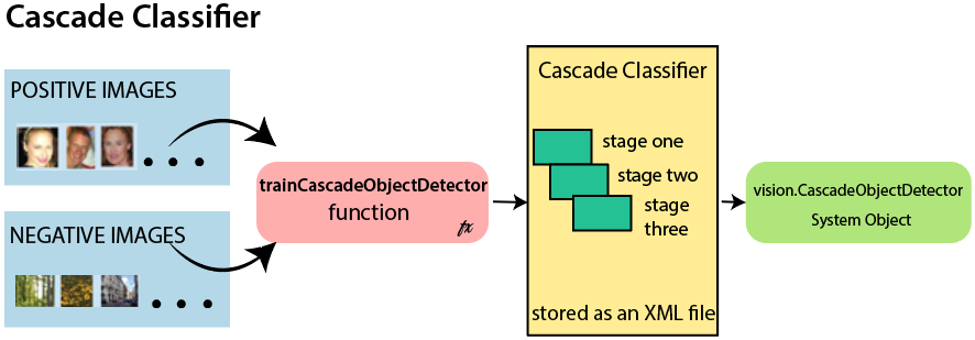
The HAAR cascade is a machine learning approach where a cascade function is trained from a lot of positive and negative images. Positive images are those images that consist of faces, and negative images are without faces. In face detection, image features are treated as numerical information extracted from the pictures that can distinguish one image from another.

We apply every feature of the algorithm on all the training images. Every image is given equal weight at the starting. It founds the best threshold which will categorize the faces to positive and negative. There may be errors and misclassifications. We select the features with a minimum error rate, which means these are the features that best classifies the face and non-face images.

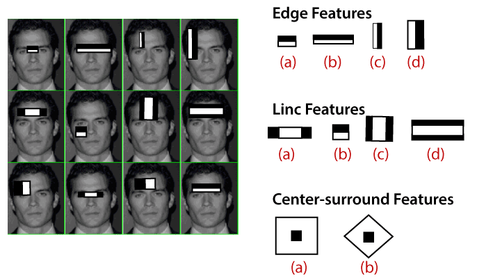
All possible sizes and locations of each kernel are used to calculate the plenty of features.

HAAR-Cascade Detection in OpenCV

OpenCV provides the trainer as well as the detector. We can train the classifier for any object like cars, planes, and buildings by using the OpenCV. There are two primary states of the cascade image classifier first one is training and the other is detection.

OpenCV provides two applications to train cascade classifier opencv_haartraining and opencv_traincascade. These two applications store the classifier in the different file format.

For training, we need a set of samples. There are two types of samples:

• Negative sample: It is related to non-object images.
• Positive samples: It is a related image with detect objects.

A set of negative samples must be prepared manually, whereas the collection of positive samples are created using the opencv_createsamples utility.

Negative Sample

Negative samples are taken from arbitrary images. Negative samples are added in a text file. Each line of the file contains an image filename (relative to the directory of the description file) of the negative sample. This file must be created manually. Defined images may be of different sizes.

Positive Sample

Positive samples are created by opencv_createsamples utility. These samples can be created from a single image with an object or from an earlier collection. It is important to remember that we require a large dataset of positive samples before you give it to the mentioned utility because it only applies the perspective transformation.

Here we will discuss detection. OpenCV already contains various pre-trained classifiers for face, eyes, smile, etc. Those XML files are stored in opencv/data/haarcascades/ folder. Let’s understand the following steps:

Step – 1

First, we need to load the necessary XML classifiers and load input images (or video) in grayscale mode.

Step -2

After converting the image into grayscale, we can do the image manipulation where the image can be resized, cropped, blurred, and sharpen if required. The next step is image segmentation; identify the multiple objects in the single image, so the classifier quickly detects the objects and faces in the picture.

Step – 3

The haar-Like feature algorithm is used to find the location of the human faces in frame or image. All the Human faces have some common universal properties of faces like the eye region is darker than it’s neighbor’s pixels and nose region is more bright than the eye region.

Step -4

In this step, we extract the features from the image, with the help of edge detection, line detection, and center detection. Then provide the coordinate of x, y, w, h, which makes a rectangle box in the picture to show the location of the face. It can make a rectangle box in the desired area where it detects the face.

Face recognition using OpenCV

Face recognition is a simple task for humans. Successful face recognition tends to effective recognition of the inner features (eyes, nose, mouth) or outer features (head, face, hairline). Here the question is that how the human brain encode it?

David Hubel and Torsten Wiesel show that our brain has specialized nerve cells responding to unique local feature of the scene, such as lines, edges angle, or movement. Our brain combines the different sources of information into the useful patterns; we don’t see the visual as scatters. If we define face recognition in the simple word, “Automatic face recognition is all about to take out those meaningful features from an image and putting them into a useful representation then perform some classification on them”.

The basic idea of face recognition is based on the geometric features of a face. It is the feasible and most intuitive approach for face recognition. The first automated face recognition system was described in the position of eyes, ears, nose. These positioning points are called features vector (distance between the points).

The face recognition is achieved by calculating the Euclidean distance between feature vectors of a probe and reference image. This method is effective in illumination change by its nature, but it has a considerable drawback. The correct registration of the maker is very hard.

The face recognition system can operate basically in two modes:

• Authentication or Verification of a facial image-

It compares the input facial image with the facial image related to the user, which is required authentication. It is a 1×1 comparison.

• Identification or facial recognition

It basically compares the input facial images from a dataset to find the user that matches that input face. It is a 1xN comparison.

There are various types of face recognition algorithms, for example:

• Eigenfaces (1991)
• Local Binary Patterns Histograms (LBPH) (1996)
• Fisherfaces (1997)
• Scale Invariant Feature Transform (SIFT) (1999)
• Speed Up Robust Features (SURF) (2006)

Each algorithm follows the different approaches to extract the image information and perform the matching with the input image. Here we will discuss the Local Binary Patterns Histogram (LBPH) algorithm which is one of the oldest and popular algorithm.

Introduction of LBPH

Local Binary Pattern Histogram algorithm is a simple approach that labels the pixels of the image thresholding the neighborhood of each pixel. In other words, LBPH summarizes the local structure in an image by comparing each pixel with its neighbors and the result is converted into a binary number. It was first defined in 1994 (LBP) and since that time it has been found to be a powerful algorithm for texture classification.

This algorithm is generally focused on extracting local features from images. The basic idea is not to look at the whole image as a high-dimension vector; it only focuses on the local features of an object.

In the above image, take a pixel as center and threshold its neighbor against. If the intensity of the center pixel is greater-equal to its neighbor, then denote it with 1 and if not then denote it with 0.

Let’s understand the steps of the algorithm:

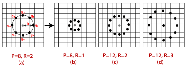
1. Selecting the Parameters: The LBPH accepts the four parameters:

• Radius: It represents the radius around the central pixel. It is usually set to 1. It is used to build the circular local binary pattern.
• Neighbors: The number of sample points to build the circular binary pattern.
• Grid X: The number of cells in the horizontal direction. The more cells and finer grid represents, the higher dimensionality of the resulting feature vector.
• Grid Y: The number of cells in the vertical direction. The more cells and finer grid represents, the higher dimensionality of the resulting feature vector.

Note: The above parameters are slightly confusing. It will be more clear in further steps.

2. Training the Algorithm: The first step is to train the algorithm. It requires a dataset with the facial images of the person that we want to recognize. A unique ID (it may be a number or name of the person) should provide with each image. Then the algorithm uses this information to recognize an input image and give you the output. An Image of particular person must have the same ID. Let’s understand the LBPH computational in the next step.

3. Using the LBP operation: In this step, LBP computation is used to create an intermediate image that describes the original image in a specific way through highlighting the facial characteristic. The parameters radius and neighbors are used in the concept of sliding window.

To understand in a more specific way, let’s break it into several small steps:

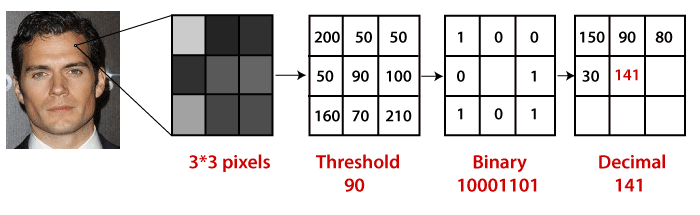
• Suppose the input facial image is grayscale.
• We can get part of this image as a window of 3×3 pixels.
• We can use the 3×3 matrix containing the intensity of each pixel (0-255).
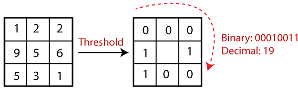
• Then, we need to take the central value of the matrix to be used as a threshold.
• This value will be used to define the new values from the 8 neighbors.
• For every neighbor of the central value (threshold), we set a new binary value. The value 1 is set for equal or higher than the threshold and 0 for values lower than the threshold.
• Now the matrix will consist of only binary values (skip the central value). We need to take care of each binary value from each position from the matrix line by line into new binary values (10001101). There are other approaches to concatenate the binary values (clockwise direction), but the final result will be the same.
• We convert this binary value to decimal value and set it to the central value of the matrix, which is a pixel from the original image.
• After completing the LBP procedure, we get the new image, which represents better characteristics of the original image.

4. Extracting the Histograms from the image: The image is generated in the last step, we can use the Grid X and Grid Y parameters to divide the image into multiple grids, let’s consider the following image:

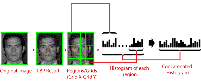
• We have an image in grayscale; each histogram (from each grid) will contain only 256 positions representing the occurrence of each pixel intensity.
• It is required to create a new bigger histogram by concatenating each histogram.

5. Performing face recognition: Now, the algorithm is well trained. The extracted histogram is used to represent each image from the training dataset. For the new image, we perform steps again and create a new histogram. To find the image that matches the given image, we just need to match two histograms and return the image with the closest histogram.

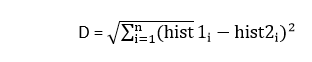
• There are various approaches to compare the histograms (calculate the distance between two histograms), for example: Euclidean distance, chi-square, absolute value, etc. We can use the Euclidean distance based on the following formula:

• The algorithm will return ID as an output from the image with the closest histogram. The algorithm should also return the calculated distance that can be called confidence measurement. If the confidence is lower than the threshold value, that means the algorithm has successfully recognized the face.

We have discussed the face detection and face recognition. The haar like cascade algorithm is used for face detection. There are various algorithms for face recognition, but LBPH is easy and popular algorithm among them. It generally focuses on the local features in the image.

---