How to Average Filtered Rows in Google Sheets (With Example)

by Tutor Aspire January 17, 2023

The easiest way to take the average of a filtered range in Google Sheets is to use the following syntax:

SUBTOTAL(101, A1:A10)

Note that the value 101 is a shortcut for taking the average of a filtered range of rows.

The following example shows how to use this function in practice.

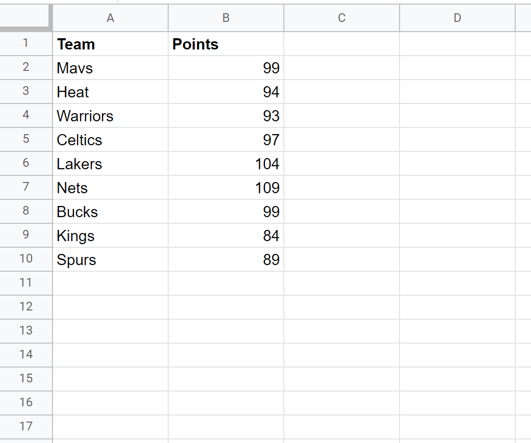
Suppose we have the following spreadsheet that contains information about various basketball teams:

To add a filter to this data, we can highlight cells A1:B10, then click the Data tab, then click Create a filter:

We can then click the Filter icon at the top of the Points column and uncheck the box next to the first three values 84, 89, and 93:

Once we click OK, the data will be filtered to remove these values.

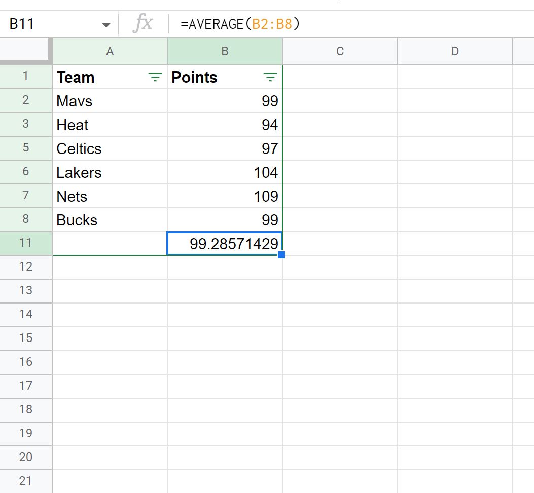
If we attempt to use the AVERAGE() function to average the points column of the filtered rows, it will not return the correct value:

Instead, need to use the SUBTOTAL() function:

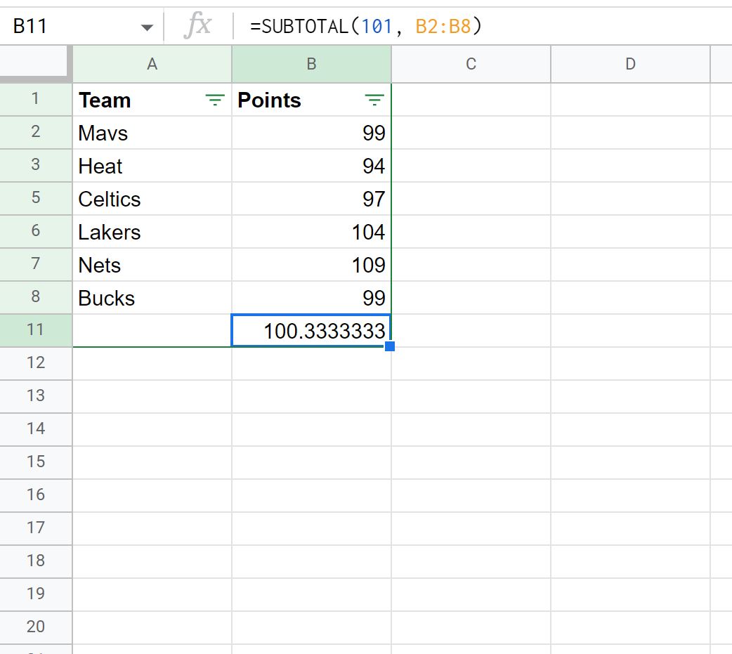
This function takes the average of only the visible rows.

We can manually verify this by calculating the average of the visible rows:

Average of Visible Rows: (99 + 94 + 97 + 104 + 109 + 99) / 6 = 100.333.

The following tutorials explain how to perform other common operations in Google Sheets: