How to Perform Logistic Regression in Python (Step-by-Step)

---

Logistic regression is a method we can use to fit a regression model when the response variable is binary.

Logistic regression uses a method known as maximum likelihood estimation to find an equation of the following form:

log[p(X) / (1-p(X))]  =  β₀ + β₁X₁ + β₂X₂ + … + β_pX_p

where:

• X_j: The j^th predictor variable
• β_j: The coefficient estimate for the j^th predictor variable

The formula on the right side of the equation predicts the log odds of the response variable taking on a value of 1.

Thus, when we fit a logistic regression model we can use the following equation to calculate the probability that a given observation takes on a value of 1:

p(X) = e^{β₀ + β₁X₁ + β₂X₂ + … + β_pX_p} / (1 + e^{β₀ + β₁X₁ + β₂X₂ + … + β_pX_p})

We then use some probability threshold to classify the observation as either 1 or 0.

For example, we might say that observations with a probability greater than or equal to 0.5 will be classified as “1” and all other observations will be classified as “0.”

This tutorial provides a step-by-step example of how to perform logistic regression in R.

Step 1: Import Necessary Packages

First, we’ll import the necessary packages to perform logistic regression in Python:

import pandas as pd
import numpy as np
from sklearn.model_selection import train_test_split
from sklearn.linear_model import LogisticRegression
from sklearn import metrics
import matplotlib.pyplot as plt

Step 2: Load the Data

For this example, we’ll use the Default dataset from the Introduction to Statistical Learning book. We can use the following code to load and view a summary of the dataset:

#import dataset from CSV file on Github
url = "https://raw.githubusercontent.com/Statology/Python-Guides/main/default.csv"
data = pd.read_csv(url)

#view first six rows of dataset
data[0:6]

        default	student	balance	        income
0	0	0	729.526495	44361.625074
1	0	1	817.180407	12106.134700
2	0	0	1073.549164	31767.138947
3	0	0	529.250605	35704.493935
4	0	0	785.655883	38463.495879
5	0	1	919.588530	7491.558572  

#find total observations in dataset
len(data.index)

10000

This dataset contains the following information about 10,000 individuals:

• default: Indicates whether or not an individual defaulted.
• student: Indicates whether or not an individual is a student.
• balance: Average balance carried by an individual.
• income: Income of the individual.

We will use student status, bank balance, and income to build a logistic regression model that predicts the probability that a given individual defaults.

Step 3: Create Training and Test Samples

Next, we’ll split the dataset into a training set to train the model on and a testing set to test the model on.

#define the predictor variables and the response variable
X = data[['student', 'balance', 'income']]
y = data['default']

#split the dataset into training (70%) and testing (30%) sets
X_train,X_test,y_train,y_test = train_test_split(X,y,test_size=0.3,random_state=0)  

Step 4: Fit the Logistic Regression Model

Next, we’ll use the LogisticRegression() function to fit a logistic regression model to the dataset:

#instantiate the model
log_regression = LogisticRegression()

#fit the model using the training data
log_regression.fit(X_train,y_train)

#use model to make predictions on test data
y_pred = log_regression.predict(X_test)

Step 5: Model Diagnostics

Once we fit the regression model, we can then analyze how well our model performs on the test dataset.

First, we’ll create the confusion matrix for the model:

cnf_matrix = metrics.confusion_matrix(y_test, y_pred)
cnf_matrix

array([[2886,    1],
       [ 113,    0]])

From the confusion matrix we can see that:

• #True positive predictions: 2886
• #True negative predictions: 0
• #False positive predictions: 113
• #False negative predictions: 1

We can also obtain the accuracy of the model, which tells us the percentage of correction predictions the model made:

print("Accuracy:",metrics.accuracy_score(y_test, y_pred))l

Accuracy: 0.962

This tells us that the model made the correct prediction for whether or not an individual would default 96.2% of the time.

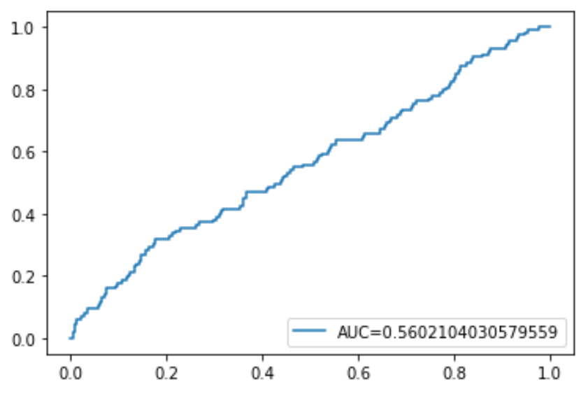
Lastly, we can plot the ROC (Receiver Operating Characteristic) Curve which displays the percentage of true positives predicted by the model as the prediction probability cutoff is lowered from 1 to 0.

The higher the AUC (area under the curve), the more accurately our model is able to predict outcomes:

#define metrics
y_pred_proba = log_regression.predict_proba(X_test)[::,1]
fpr, tpr, _ = metrics.roc_curve(y_test,  y_pred_proba)
auc = metrics.roc_auc_score(y_test, y_pred_proba)

#create ROC curve
plt.plot(fpr,tpr,label="AUC="+str(auc))
plt.legend(loc=4)
plt.show()