Multiple linear regression is a statistical method we can use to understand the relationship between multiple predictor variables and a response variable.
However, one of the key assumptions of multiple linear regression is that there exists a linear relationship between each predictor variable and the response variable.
If this assumption is violated, then the results of the regression model can be unreliable.
One way to check this assumption is to create a partial residual plot, which displays the residuals of one predictor variable against the response variable.
The following example shows how to create partial residual plots for a regression model in R.
Example: How to Create Partial Residual Plots in R
Suppose we fit a regression model with three predictor variables in R:
#make this example reproducible
set.seed(0)

#define response variable
y #define three predictor variables
x1 #fit multiple linear regression model
model
We can use the crPlots() function from the car package in R to create partial residual plots for each predictor variable in the model:
library(car)

#create partial residual plots
crPlots(model)
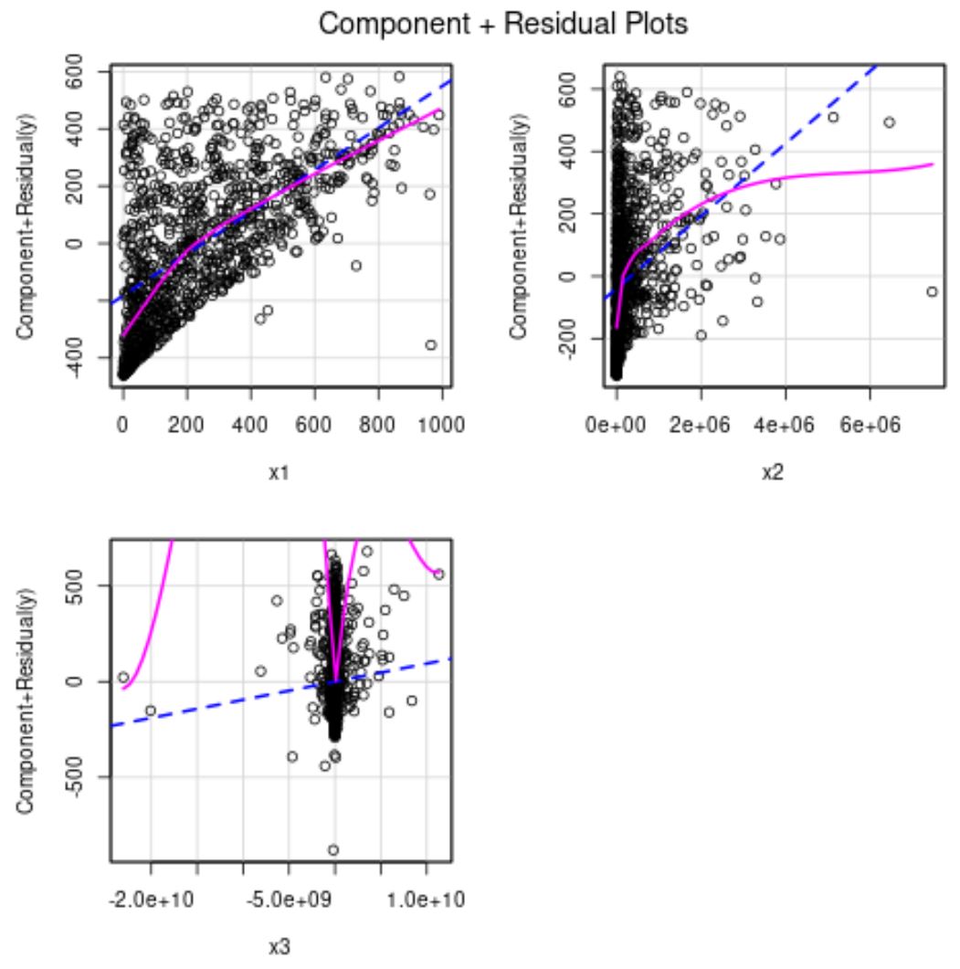
The blue line shows the expected residuals if the relationship between the predictor and response variable was linear. The pink line shows the actual residuals.
If the two lines are significantly different, then this is evidence of a nonlinear relationship.
From the plots above we can see that the residuals for both x2 and x3 appear to be nonlinear.
This violates the assumption of linearity for multiple linear regression. One way to fix this issue is to use a square root or cubic transformation on the predictor variables:
library(car)

#fit new model with transformed predictor variables
model_transformed #create partial residual plots for new model
crPlots(model_transformed)

From the partial residual plots we can see that x2 now has a more linear relationship with the response variable.
The predictor variable x3 is still somewhat nonlinear so we may decide to try another transformation or possibly drop the variable from the model altogether.
Additional Resources
The following tutorials explain how to create other common plots in R:
How to Create Diagnostic Plots in R
How to Create a Scale-Location Plot in R
How to Create a Residual Plot in R