T-Test in Python
An Introduction
As we all know, Python provides various Statistics Libraries, in which some are pretty popular such as PyMC3 and SciPy. These libraries provide users different pre-defined functions in order to compute various tests. But in order to understand the mathematics behind the process, it is imperious to understand what is happening in the background. In the following tutorial, we will understand how to perform a T-test in Python using NumPy.
A T-test is among the most frequently utilized procedures in statistics. However, many people who even use T-test frequently do not precisely know what happens to their data when wheeled away and operated upon in the background using the applications such as R and Python.
But before we get started, let us understand what the T-test is.
Understanding T-test
The T-test is the test that compares two averages, also known as means, and tells us whether they differ from each other or not. The T-test is also known as Student’s T-test, and it also tells us how significant the differences are. In other terms, it provides us knowledge of whether those differences could have occurred by chance.
Now, let us understand some examples.
Suppose we have a fever and we try a naturalistic medication. The fever lasts for some days. The next time we have a fever, we go to the medical store and buy an over-the-counter pharmaceutical. This time the fever lasts for a week. When we survey our friends, we found out that their fever lasted for a shorter time (an average of 3 days) when they took the homeopathic medication. In this survey, what we need to know is, are these outcomes repeatable? A T-test will let us know the means of the two groups by comparing and also the probability of those outcomes occurring by chance.
We can also use Student’s T-test in real life in order to compare means. For instance, a drug company wants to test a new cancer drug in order to check its improvement in life expectancy. In an experiment, there is generally a control group (A group that is provided with a ‘sugar pill” or placebo). The control group may display a mean life expectancy of more than five years, whereas the group consuming the new drug might have a life expectancy of more than six years. As a result, we can say that the drug might work; however, there is a chance it could be because of a fluke. Thus, to test this, researchers will utilize a Student’s T-test in order to find out whether the outcomes are repeatable for a whole population or not.
Now, let us understand what T-score is.
Understanding T-score
A Ratio between the difference between two groups and the difference within the groups is known as the T-score. If the T-score is more significant, this means that there is more difference present between the groups. At the same time, the smaller T-score signifies the similarities between the groups. A T-score of Three (3) indicates that the group is three times different from each other and within each other. When we get a bigger T-value while running a T-test, it more list that the outcomes are repeatable.
Thus, we can conclude that the following:
- A large T-score implies that the groups are different from each other.
- A small T-score implies that the groups are similar.
Now, let us understand the T-values and P-values.
Understanding T-values and P-values
Every T-value contains a P-value to work with it. A P-value is referred to as the probability that the outcomes from the sample data happened coincidentally. P-values have values starting from 0% to 100%. They are generally written as a decimal. For instance, a P-value of 10% is 0.1. It is good to have low P-values. Lower P-values indicate that the data did not happen coincidentally. For instance, a P-value of 0.1 indicates that there is only a 1% probability that the experiment’s outcomes occurred coincidentally. Generally, in many cases, a P-value of 5%, that is 0.05, is accepted to mean the data is said to be valid.
Now, let us understand the types of T-tests.
What are the Types of T-tests?
There are Three significant Types of T-test:
- Independent Samples T-test: This test is used to compare the averages or means for two groups.
- Paired Sample T-test: This test is used to compare means from the same group at different times (For example, one year apart).
- One Sample T-test: This test is used to test the mean of a single group against an acknowledged mean.
Now, let us start performing a sample T-test.
Performing a Sample T-test
Suppose that we need to test if the men’s height in the population differs from the women’s height in general. Thus, we will take a sample from the population and utilize the T-test to check whether the result is significant or not.
We will follow the steps given below:
Step 1: Determining a Null and Alternate Hypothesis
Step 2: Collecting Sample data
Step 3: Determining a Confidence Interval and Degrees of Freedom
Step 4: Calculating the T-Statistics
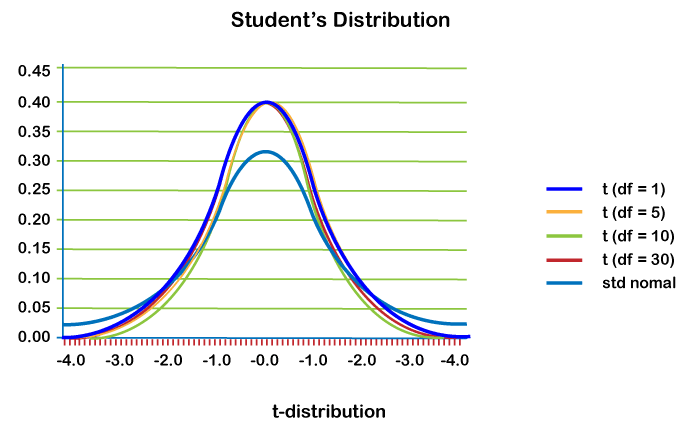
Step 5: Calculating the critical T-value from the T-Distribution
Step 6: Comparing the critical T-values with the calculated T-Statistics
Let us begin understanding the above steps in brief.
Determining a null and alternate hypothesis
Starting with defining a null and alternate hypothesis is necessary. In general, the null hypothesis will express that the two being tested populations have no significant difference statistically. On the other hand, the alternate hypothesis will express that there is one present. For this example, we can conclude the following statements:
- Null Hypothesis: The height of men & women is the same.
- Alternate Hypothesis: The height of men differs from the height of women.
Collecting sample data
Once we determined the hypothesis, we will start collecting the data from each population group. For this example, we will be collecting two sets of data. The one data set containing the height of men and the other one with the height of men. The size of sample data ideally needs to be identical; however, it can be different. Suppose that the sizes of sample data are nx and ny.
Determining a Confidence interval and degrees of freedom
Confidence interval is generally called alpha (α). The typical value of alpha (α) is 0.05. This statement implies that there is 95% confidence for the valid conclusion of the test. We can define the degree of freedom by using the formula given below:

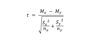
Calculating the T-Statistic
We can calculate the t-statistic by using the following formula:
M = mean
n = number of scores per group
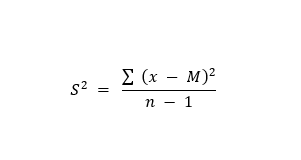
x = individual scores
M = mean
n = number of scores in group
Moreover, Mx and My are the values of the mean of the two female and male samples. Nx and Ny are the sample space of the two samples, and S is the standard deviation.
Calculating the critical T-value from the T-Distribution
We require two objects in order to calculate the critical t-value. The first is the alpha’s chosen value, and the other is the degrees of freedom. The formula of critical t-value is complex; however, it is static for a fixed degree of freedom pair and the alpha’s value. We thus, utilize a table in order to calculate the critical t-value.
However, Python provides a function in the SciPy library that serves the same purpose.
Comparing the critical T-values with the calculated T-Statistic
Once the critical T-value is calculated, we will compare the value with the T-Statistic that we have calculated earlier. If the critical t-value is less than the calculated T-Statistic, the test deduces that a significant difference is present between the two populations statistically. Hence, we have to reject the null hypothesis that no significant difference is present between the two samples statistically.
However, in another case where there is no significant difference between the two populations, the test fails to reject the null hypothesis. Thus, we accept the alternate hypothesis implying that the men’s and women’s height are statistically different.
Let us consider the following Python program demonstrating the working of the model.
Program:
Output:
Standard Deviation = 0.7642398582227466 t = 4.87688162540348 p = 0.0001212767169695983 t = 4.876881625403479 p = 0.00012127671696957205
Explanation:
In the above example, we have imported the required libraries and defined the variable containing the sample size of the data. We have then calculated the Gaussian Distributed Data and Standard Deviation. After that, we have calculated the T-Statistic and compared it with the critical T-value. For this, we have calculated the degrees of freedom and compare the p-value. Once the comparison is made, we have printed the values for the users. At last, we have used the function of the SciPy package to compare the values again and printed them.