Multicollinearity in regression analysis occurs when two or more predictor variables are highly correlated to each other, such that they do not provide unique or independent information in the regression model.
If the degree of correlation is high enough between variables, it can cause problems when fitting and interpreting the regression model.
The most common way to detect multicollinearity is by using the variance inflation factor (VIF), which measures the correlation and strength of correlation between the predictor variables in a regression model.
The value for VIF starts at 1 and has no upper limit. A general rule of thumb for interpreting VIFs is as follows:
- A value of 1 indicates there is no correlation between a given predictor variable and any other predictor variables in the model.
- A value between 1 and 5 indicates moderate correlation between a given predictor variable and other predictor variables in the model, but this is often not severe enough to require attention.
- A value greater than 5 indicates potentially severe correlation between a given predictor variable and other predictor variables in the model. In this case, the coefficient estimates and p-values in the regression output are likely unreliable.
Note that there are some cases in which high VIF values can safely be ignored.
How to Calculate VIF in R
To illustrate how to calculate VIF for a regression model in R, we will use the built-in dataset mtcars:
#view first six lines of mtcars
head(mtcars)

#                   mpg cyl disp  hp drat    wt  qsec vs am gear carb
#Mazda RX4         21.0   6  160 110 3.90 2.620 16.46  0  1    4    4
#Mazda RX4 Wag     21.0   6  160 110 3.90 2.875 17.02  0  1    4    4
#Datsun 710        22.8   4  108  93 3.85 2.320 18.61  1  1    4    1
#Hornet 4 Drive    21.4   6  258 110 3.08 3.215 19.44  1  0    3    1
#Hornet Sportabout 18.7   8  360 175 3.15 3.440 17.02  0  0    3    2
#Valiant           18.1   6  225 105 2.76 3.460 20.22  1  0    3    1
First, we’ll fit a regression model using mpg as the response variable and disp, hp, wt, and drat as the predictor variables:
#fit the regression model
model #view the output of the regression model
summary(model)

#Call:
#lm(formula = mpg ~ disp + hp + wt + drat, data = mtcars)
#
#Residuals:
#    Min      1Q  Median      3Q     Max
#-3.5077 -1.9052 -0.5057  0.9821  5.6883
#
#Coefficients:
#             Estimate Std. Error t value Pr(>|t|)
#(Intercept) 29.148738   6.293588   4.631  8.2e-05 ***
#disp         0.003815   0.010805   0.353  0.72675
#hp          -0.034784   0.011597  -2.999  0.00576 **
#wt          -3.479668   1.078371  -3.227  0.00327 **
#drat         1.768049   1.319779   1.340  0.19153
#---
#Signif. codes:  0 '***' 0.001 '**' 0.01 '*' 0.05 '.' 0.1 ' ' 1
#
#Residual standard error: 2.602 on 27 degrees of freedom
#Multiple R-squared:  0.8376,	Adjusted R-squared:  0.8136
#F-statistic: 34.82 on 4 and 27 DF,  p-value: 2.704e-10
We can see from the output that the R-squared value for the model is 0.8376. We can also see that the overall F-statistic is 34.82 and the corresponding p-value is 2.704e-10, which indicates that the overall regression model is significant. Also, the predictor variables hp and wt are statistically significant at the 0.05 significance level while disp and drat are not.
Next, we’ll use the vif() function from the car library to calculate the VIF for each predictor variable in the model:
#load the car library
library(car)

#calculate the VIF for each predictor variable in the model
vif(model)

#    disp       hp       wt     drat
#8.209402 2.894373 5.096601 2.279547
We can see that the VIF for both disp and wt are greater than 5, which is potentially concerning.
Visualizing VIF Values
To visualize the VIF values for each predictor variable, we can create a simple horizontal bar chart and add a vertical line at 5 so we can clearly see which VIF values exceed 5:
#create vector of VIF values
vif_values #create horizontal bar chart to display each VIF value
barplot(vif_values, main = "VIF Values", horiz = TRUE, col = "steelblue")

#add vertical line at 5
abline(v = 5, lwd = 3, lty = 2)
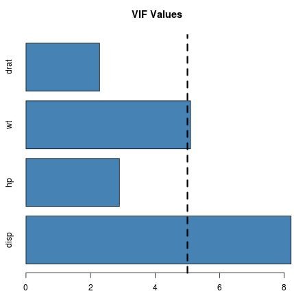
Note that this type of chart would be most useful for a model that has a lot of predictor variables, so we could easily visualize all of the VIF values at once. It is still a useful chart in this example, though.
Depending on what value of VIF you deem to be too high to include in the model, you may choose to remove certain predictor variables and see if the corresponding R-squared value or standard error of the model is affected.
Visualizing Correlations Between Predictor Variables
To gain a better understanding of why one predictor variable may have a high VIF value, we can create a correlation matrix to view the linear correlation coefficients between each pair of variables:
#define the variables we want to include in the correlation matrix
data #create correlation matrix
cor(data)

#           disp         hp         wt       drat
#disp  1.0000000  0.7909486  0.8879799 -0.7102139
#hp    0.7909486  1.0000000  0.6587479 -0.4487591
#wt    0.8879799  0.6587479  1.0000000 -0.7124406
#drat -0.7102139 -0.4487591 -0.7124406  1.0000000
Recall that the variable disp had a VIF value over 8, which was the largest VIF value among all of the predictor variables in the model. From the correlation matrix we can see that disp is strongly correlated with all three of the other predictor variables, which explains why it has such a high VIF value.
In this case, you may want to remove disp from the model because it has a high VIF value and it was not statistically significant at the 0.05 significance level.
Note that a correlation matrix and a VIF will provide you with similar information: they both tell you when one variable is highly correlated with one or more other variables in a regression model.
Further Reading:
A Guide to Multicollinearity & VIF in Regression
What is a Good R-squared Value?