Linear Regression in TensorFlow

Linear Regression is a machine learning algorithm that is based on supervised learning. It performs a regression function. The regression models a target predictive value based on the independent variable. It is mostly used to detect the relation between variables and forecasts.

Linear regression is a linear model; for example, a model that assumes a linear relationship between an input variable (x) and a single output variable (y). In particular, y can be calculated by a linear combination of input variables (x).

Linear regression is a prevalent statistical method that allows us to learn a function or relation from a set of continuous data. For example, we are given some data point of x and the corresponding, and we need to know the relationship between them, which is called the hypothesis.

In the case of linear regression, the hypothesis is a straight line, that is,

h (x) = wx + b

Where w is a vector called weight, and b is a scalar called Bias. Weight and bias are called parameters of the model.

We need to estimate the value of w and b from the set of data such that the resultant hypothesis produces at least cost ‘j,’ which has been defined by the below cost function.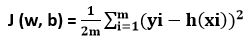

Where m is the data points in the particular dataset.

This cost function is called the Mean Squared Error.

For optimization of parameters for which the value of j is minimal, we will use a commonly used optimizer algorithm, called gradient descent. The following is pseudocode for gradient descent:

Where ? is a hyperparameter which called the learning rate.

Implementation of Linear Regression

We will start to import the necessary libraries in Tensorflow. We will use Numpy with Tensorflow for computation and Matplotlib for plotting purposes.

First, we have to import packages:

To make the random numbers predicted, we have to define fixed seeds for both Tensorflow and Numpy.

Now, we have to generate some random data for training the Linear Regression Model.

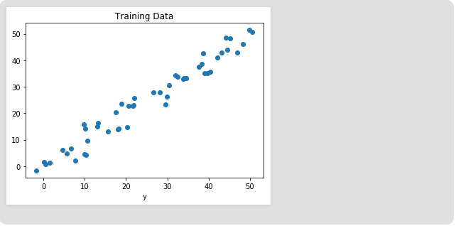
  # Generating random linear data   # There will be 50 data points which are ranging from 0 to 50.  x = np.linspace(0, 50, 50)   y = np.linspace(0, 50, 50)       # Adding noise to the random linear data   x += np.random.uniform(-4, 4, 50)   y += np.random.uniform(-4, 4, 50)   n= len(x) #Number of data points  

Let us visualize the training data.

# Plot of Training Data

  plt.scatter(x, y)   plt.xlabel(‘x’)   plt.xlabel(‘y’)   plt.title(“Training Data”)   plt.show()   

Output

Now, we will start building our model by defining placeholders x and y, so that we feed the training examples x and y into the optimizer while the training process.

Now, we can declare two trainable TensorFlow variables for the bias and Weights initializing them randomly using the method:

  np.random.randn().  W= tf.Variable(np.random.randn(), name=”W”)  B= tf.Variable(np.random,randn(), name=”b”)  

Now we define the hyperparameter of the model, the learning rate and the number of Epochs.

Now, we will build Hypothesis, Cost Function and Optimizer. We will not manually implement the Gradient Decent Optimizer because it is built inside TensorFlow. After that, we will initialize the variables in the method.

  # Hypothesis of the function  y_pred = tf.add(tf.multiply(X, W), b)   # Mean Square Error function        cost = tf.reduce_sum(tf.pow(y_pred-Y, 2)) / (2 * n)    # Gradient Descent Optimizer function  optimizer = tf.train.GradientDescentOptimizer (learning_rate).minimize(cost)  # Global Variables Initializer   init = tf.global_variables_initializer( )  

Now we start the training process inside the TensorFlow Session.

  # Starting the Tensorflow Session   with tf.Session() as sess:              # Initializing the Variables       sess.run(init)              # Iterating through all the epochs       for epoch in range(training_epochs):                   # Feeding each data point into the optimizer according to the Feed Dictionary.    for (_x, _y) in zip(x, y):      sess.run(optimizer, feed_dict = {X : _x, Y : _y})       # Here, we are displaying the result after every 50 epoch            if (epoch + 1) % 50 ==0:    # Calculating the cost at every epoch.    c = sess.run(cost, feed_dict = {X : x, Y : y})    print(“Epoch”, (epoch + 1), “: cost =”, c, “W =”, sess.run(W), “b=”, sess.run(b))   # Store the necessary value which has used outside the Session       training_cost = sess.run (cost, feed_dict ={X: x, Y: y})        weight = sess.run(W)       bias = sess.run(b)   

Output is given below:

Epoch: 50  cost = 5.8868037 W = 0.9951241 b = 1.2381057  Epoch: 100 cost = 5.7912708 W = 0.9981236 b = 1.0914398  Epoch: 150 cost = 5.7119676 W = 1.0008028 b = 0.96044315  Epoch: 200 cost = 5.6459414 W = 1.0031956 b = 0.8434396  Epoch: 250 cost = 5.590798 W = 1.0053328 b = 0.7389358  Epoch: 300 cost = 5.544609 W = 1.007242 b = 0.6455922  Epoch: 350 cost = 5.5057884 W = 1.008947 b = 0.56223  Epoch: 400 cost = 5.473068 W = 1.01047 b = 0.46775345  Epoch: 450 cost = 5.453845 W = 1.0118302 b = 0.42124168  Epoch: 500 cost = 5.421907 W = 1.0130452 b = 0.36183489  Epoch: 550 cost = 5.4019218 W = 1.0141305 b = 0.30877414  Epoch: 600 cost = 5.3848578 W = 1.0150996  b = 0.26138115  Epoch: 650 cost = 5.370247 W = 1.0159653  b = 0.21905092  Epoch: 700 cost = 5.3576995 W = 1.0167387  b = 0.18124212  Epoch: 750 cost = 5.3468934 W = 1.0174294  b = 0.14747245  Epoch: 800 cost = 5.3375574 W = 1.0180461  b = 0.11730932  Epoch: 850 cost = 5.3294765 W = 1.0185971  b = 0.090368526  Epoch: 900 cost = 5.322459 W = 1.0190894  b = 0.0663058  Epoch: 950 cost = 5.3163588 W = 1.0195289  b = 0.044813324  Epoch: 1000 cost = 5.3110332 W = 1.0199218  b = 0.02561669

Now, see the result.

  # Calculate the predictions  predictions = weight * x + bias   print (“Training cost =”, training_cost, “Weight =”, weight, “bias =”, bias, ‘n’)   

Output

Training cost= 5.3110332 Weight= 1.0199214 bias=0.02561663

Note that in this case, both weight and bias are scalars in order. This is because we have examined only one dependent variable in our training data. If there are m dependent variables in our training dataset, the weight will be a one-dimensional vector while Bias will be a scalar.

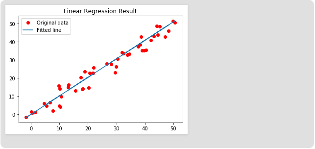
Finally, we will plotting our result:

  # Plotting the Results below  plt.plot(x, y, ‘ro’, label =’original data’)  plt.plot(x, predictions, label =’Fited line’)  plt.title(‘Linear Regression Result’)   plt.legend()   plt.show()   

Output

Next TopicCNN Introduction

advantages of tensorflow disadvantages of tensorflow installation of tensorflow through conda installation of tensorflow through pip pros and cons of tensorflow tensorflow tensorflow architecture tensorflow installation tensorflow introduction tensorflow overview tensorflow tutorial what is tensorflow

Linear Regression in TensorFlow

Linear Regression in TensorFlow

Implementation of Linear Regression

Tableau Tutorial | Data Visualization Tool

Exclude Include Test Cases in TestNG

You may also like