76

Stability conditions

The essential requirement for the control system is that it should be stable. It means that the output of the system should follow the input. If the input is finite, the output also needs to be finite in order to satisfy the stability condition.

An LTI (Linear Time-Invariant) system should be stable under the following conditions:

1. BIBO (Bounded Input Bounded Output)
   It means that under any initial conditions, the system responds to the bounded input signal with the bounded output signal. If such a condition is satisfied, the system is said to be BIBO. It is commonly used for signal processing systems.
2. Linear input and output irrespective of the initial conditions
   It means that if the input is zero, the output should also be zero irrespective of any initial conditions.

Let us consider two systems described the following equations:

1. y(t) = x(t)
2. y(t) = {x(t)}^-1

Where,

x(t) = e^-t

The input in both cases is e^-t (inverse exponential function). The graph is shown below:

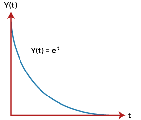
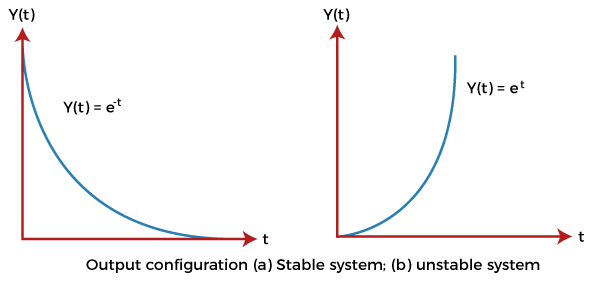
The above input is the bounded input. Now, for the condition to be stable, the output also needs to be bounded. The above graph shows that the output decreases and reaches value 0.Hence, the system is stable.

Let’s consider a case of positive exponential graph. The positive exponential graph (Y(t) = e^t) is shown below:

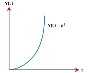
The output in this case, increases with time. It tends to infinity. When the output tends to infinity it becomes unstable.

Stability with respect to the location of poles and zeroes

In terms of poles and zeroes, we can represent the transfer function as:

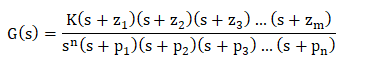
Here, z represents zeroes, and p represents poles. The value of s for which the numerator of the given transfer function is equated to zero is known as zeroes of the system. Similarly, the value of s for which the denominator of the given transfer function is equated to zero is known as the system’s pole.

The roots of the numerator can be represented as ?z1, -z2, -z3… -zm, which are known as zeroes.

The roots of the denominator can be represented as ?p1, -p2, -p3… -pn, which are known as poles. Poles are the value of s for which the transfer function is infinite. It is because it is a part of denominator. 1/infinite = 0.

Both zeroes and poles can be real or complex quantities.

Let’s consider an example.

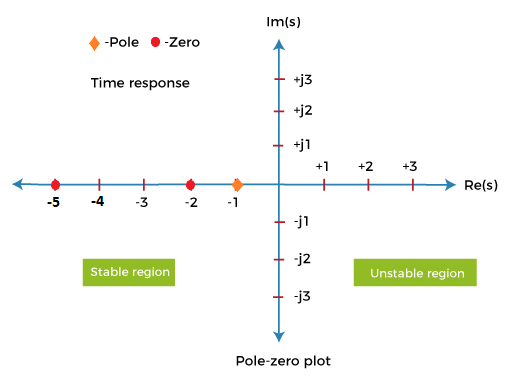
Example: G(s) = (s + 5)(s + 2)/ (s + 1)

Here, there are two terms in the numerator and one term in denominator. It means that the above transfer function includes two zeroes and one pole.

Equating numerator to 0,

(s + 5)(s + 2) = 0

s = -5, -2

Thus, the zeroes are -5 and -2.

Equating denominator to 0,

(s + 1) = 0

s = -1

Thus, the pole is -1.

The poles and zeroes are shown in the below plot.

S-Plane Plots

The s variable is equal to jw. It means that the variable s is a complex number. We can also use the value of s to construct a plot. The transfer function provides the poles and zeroes, which can be plotted graphically.

Consider the below example.

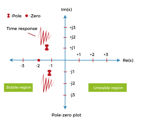
Example: G(s) = 5 (s + 2)/ s^2 + 2s + 2

Solution:

The zeroes can be obtained by equating the numerator to 0. It is given by:

5 (s + 2) = 0

S = -2

The poles are obtained by equating the denominator to 0. It is given by:

s^2 + 2s + 2 = 0

After solving, we get:

-1 + j, and -1 -j.

The pole-zero plots are shown below:

Let’s discuss the stability of the system with respect to the location of poles.

The poles with the negative real part on the left half of the s-plane are considered poles of a stale system. Thus, we can say that a stable system has a closed-loop transfer function with poles lying only in the left half of the s-plane.

A system is unstable if a pole or more than one pole is present on the right half of the s-plane or poles lying on the imaginary axis.

Before beginning with the Routh Hurwitz criteria, let’s discuss some concepts of it.

Basic concepts of Routh Hurwitz criteria

• The Routh criteria do not provide the exact locations of the roots of the characteristic equation that lie on the right-half of the s-plane. It is because the system becomes unstable if any one of the root approaches towards the right-half of the s-plane.
• It does not tell whether the roots are real or complex. The real roots are in the form of real numbers. The complex roots are represented with iota and includes the imaginary part.
• It works for only a linear system.
• It is valid if the characteristic equation is algebraic. It means that the criteria are not valid if any of the coefficients of the characteristic equation is exponential or complex.

---