Time Series in RNN

In this tutorial, we will use an RNN with time-series data. Time series is dependent on the previous time, which means past values include significant information that the network can learn. The time series prediction is to estimate the future value of any series, let’s say, stock price, temperature, GDP, and many more.

The data preparation for RNN and time-series make a little bit tricky. The objective is to predict the other value of the series, and we will use the past information to estimate the cost at t +1. The label is equal to the input succession one period along.

Secondly, the number of inputs is set to 1, i.e., one observation per time. In the end, the time step is equal to the sequence of the numerical value. If we set the time step to 10, the input sequence will return ten consecutive times.

Look at the graph below, and we have to represent the time series data on the left and a fictive input sequence on the right. We create a function to return a dataset with a random value for each day from January 2001 to December 2016

  # To plotting amazing figure   %matplotlib inline  import matplotlib  import pandas as pd  import matplotlib.pyplot as plt  def create_ts(start = ‘2001’, n = 201, freq = ‘M’):  ring = pd.date_range(start=start, periods=n, freq=freq)  ts =pd.Series(np.random.uniform(-18, 18, size=len(rng)), ring).cumsum()  return ts  ts= create_ts(start = ‘2001’, n = 192, freq = ‘M’)  ts.tail(5)  

Output:

2016-08-31    -93.459631  2016-09-30    -95.264791  2016-10-31    -95.551935  2016-11-30   -105.879611  2016-12-31   -123.729319  Freq: M, dtype: float64    ts = create_ts(start = '2001', n = 222)

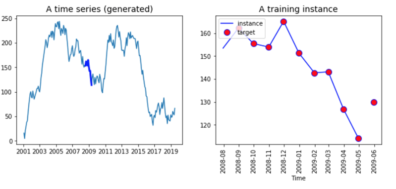
  # Left plotting diagram  plt.figure(figsize=(11,4))  plt.subplot(121)  plt.plot(ts.index, ts)  plt.plot(ts.index[90:100], ts[90:100], “b-“,linewidth=3, label=”A train illustration in the plotting area”)  plt.title(“A time series (generated)”, fontsize=14)    ## Right side plotted Diagram  plt.subplot(122)  plt.title(“A training instance”, fontsize=14)  plt.plot(ts.index[90:100], ts[90:100], “b-“, markersize=8, label=”instance”)  plt.plot(ts.index[91:101], ts[91:101], “bo”, markersize=10, label=”target”, markerfacecolor=’red’)  plt.legend(loc=”upper left”)  plt.xlabel(“Time”)  plt.show()  

The right part of the graph shows all the series. It starts in 2001 and finishes in 2019. There is no sense to makes no sense to feed all the data in the network; instead, we have to create a batch of data with a length equal to the time step. This batch will be the X variable. The Y variable is the same as the X but shifted by one period (i.e., we want to forecast t+1).

Both vectors have the same length. We can see this in the right part of the graph above. The line represents ten values of the x input, while the red dots label has ten values, y. Note that, the label starts one period forward of X and ends after one period.

Build an RNN to analyze Time Series in TensorFlow

It is time to build our first RNN to predict the series. We have to specify some hyperparameters (the parameters of the model, i.e., number of neurons, etc.) for the model.

Number of input: 1
Time step (windows in time series): 10
Number of neurons: 120
Number of output: 1

Our network will learn from a sequence of 10 days and contain 120 recurrent neurons. We feed the model with one input.

Before constructing the model, we need to split the dataset into the train set and test set. The full dataset has 222 data points; We will use the first 201 points to train the model and the last 21 points to test our model.

After we define a train and test set, we need to create an object containing the batches. In these batches, we have X values and Y values. Remember that the X value is one period straggle. Therefore, We use the first 200 observations, and the time step is equal to 10. The x_batches object must have 20 batches of size 10 or 1. The size of the Y_batches is the same as the X_batches object, but with a period above.

Step 1) Create the train and test

Firstly, we convert the series into a numpy array; then, we define the windows (the number of time networks will learn from), the number of input, output, and the size of the train set.

  series = np.array(ts)  n_windows = 20     n_input =  1  n_output = 1  size_train = 201  

After that, we split the array into two datasets.

  # Split data  train = series[:size_train]  test = series[size_train:]  print(train.shape, test.shape)  (201) (21)  

Step 2) Create the function return X_batches and y_batches

We can create a function that returns two different arrays, one for X_batches and one for y_batches. To make it easier.

Let’s make a function to construct the batches.

Note that, the X_batches are logged by one period (we take value t-1). The output of the function has three dimensions. The first dimensions are equal to the number of batches, the second is the size of the windows, and the last one is the number of input.

The tricky part of the time series is to select the data points correctly. For the X data points, we choose the observations from t = 1 to t =200, while for the Y data point, we return the observations from t = 2 to 201. Once we have the correct data points, it is effortless to reshape the series.

To construct the object with the batches, we need to split the dataset into ten batches of the same length. We can use the reshape method and pass -1 so that the series is the same as the batch size. The value 20 is the number of comments per batch, and 1 is the number of inputs.

We need to do the same step for the label.

Note that we need to shift the data to the number of times we want to forecast. For instance, if we want to predict one time, then we shift the series by 1. If we want to forecast two days, then shift the data by 2 points.

  x_data = train[:size_train-1]: Select the training instance.  X_batches = x_data.reshape(-1, Windows, input): creating the right shape for the batch.  def create_batches(df, Windows, input, output):      ## Create X                   x_data = train[:size_train-1] # Select the data          X_batches = x_data.reshape(-1, windows, input)  # Reshaping the data in this line of code      ## Create y          y_data = train[n_output:size_train]          y_batches = y_data.reshape(-1, Windows, output)          return X_batches, y_batches #return the function  

Now the function is defined, we call it for creating the batches.

  Windows = n_  Windows, # Creating windows                            input = n_input,                                        output = n_output)  

We can print the shape to make sure the dimensions are correct.

We need to create the test set with only one batch of data and 20 observations.

Note that our forecast days after days, it means the second predicted value will be based on the actual value of the first day (t+1) of the test dataset. The true value will be known.

If you want to forecast t+2, we need to use the predicted value t+1; if you’re going to predict t+3, we need to use the expected value t+1 and t+2. It makes it is difficult to predict precisely “t+n” days.

  X_test, y_test = create_batches(df = test, windows = 20,input = 1, output = 1)  print(X_test.shape, y_test.shape)  (10, 20, 1) (10, 20, 1)  

Our batch size is ready, we can build the RNN architecture. Remember, we have 120 recurrent neurons.

Step 3) Build the model

To create the model, we need to define three parts:

The variable with the tensors
The RNN
The loss and optimization

1. Variables

We need to specify the X and y variables with an appropriate shape. This step is trivial. The tensors are the same dimension as the objects X_batches and the object y_batches.

For instance, the tensors X is a placeholder has almost three dimensions:

Note: size of the batch
n_windows: Lenght of the windows.
n_input: Number of input

The result is:

  tf.placeholder(tf.float32, [None, n_windows, n_input])   ## 1. Construct the tensors  X = tf.placeholder(tf.float32, [None, n_windows, n_input])     y = tf.placeholder(tf.float32, [None, n_windows, n_output])  

2. Create the RNN

In the second part, we need to define the architecture of the network. As before, we use the object BasicRNNCell and the dynamic_rnn from TensorFlow estimator.

  ## 2. create the model  basic_cell = tf.contrib.rnn.BasicRNNCell(num_units=r_neuron, activation=tf.nn.relu)     rnn_output, states = tf.nn.dynamic_rnn(basic_cell, X, dtype=tf.float32)     

The next part is trickier but allows faster computation. We need to transform the run output to a dense layer and then convert it to has the same dimension like the input field.

  stacked_rnn_output = tf.reshape(rnn_output, [-1, r_neuron])            stacked_outputs = tf.layers.dense(stacked_rnn_output, n_output)         outputs = tf.reshape(stacked_outputs, [-1, n_windows, n_output])    

3. Create the loss and optimization

The model optimization depends on the task which we are performing.

This difference is important because it can change the optimization problem. The optimization problem for a continuous variable use to minimize the mean square error. To construct these metrics in TF, we can use:

The enduring code is the same as before; we use an Adam optimizer to reduce the loss.

We can pack everything together, and our model is ready to train.

  tf.reset_default_graph()  r_neuron = 120        ## 1. Constructing the tensors  X = tf.placeholder(tf.float32, [None, n_windows, n_input])     y = tf.placeholder(tf.float32, [None, n_windows, n_output])  

  ## 2. creating our models  basic_cell = tf.contrib.rnn.BasicRNNCell(num_units=r_neuron, activation=tf.nn.relu)     rnn_output, states = tf.nn.dynamic_rnn(basic_cell, X, dtype=tf.float32)                  stacked_rnn_output = tf.reshape(rnn_output, [-1, r_neuron])            stacked_outputs = tf.layers.dense(stacked_rnn_output, n_output)         outputs = tf.reshape(stacked_outputs, [-1, n_windows, n_output])       ## 3. Loss optimization of RNN  learning_rate = 0.001       loss = tf.reduce_sum(tf.square(outputs – y))      optimizer = tf.train.AdamOptimizer(learning_rate=learning_rate)           training_op = optimizer.minimize(loss)                                              init = tf.global_variables_initializer()   

We will train the model using 1500 epochs and print the loss every 150 iterations. Once the model is trained, we evaluate the model on the test set and create an object containing the prediction.

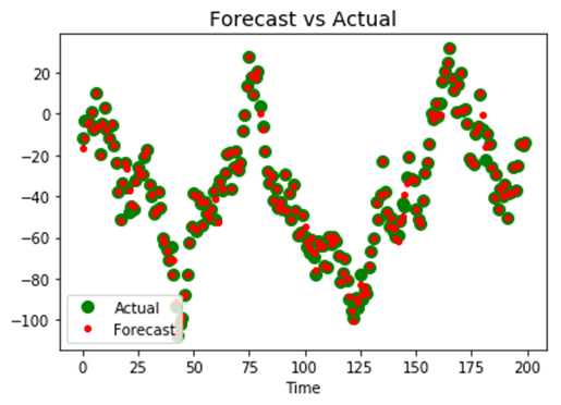
  iteration = 1500   with tf.Session() as sess:      init.run()      for iters in range(iteration):          sess.run(training_op, feed_dict={X: X_batches, y: y_batches})          if iters % 150 == 0:              mse = loss.eval(feed_dict={X: X_batches, y: y_batches})              print(iters, “tMSE:”, mse)      y_pred = sess.run(outputs, feed_dict={X: X_test})  “0 MSE: 502893.34  150 MSE: 13839.129  300 MSE: 3964.835  450 MSE: 2619.885  600 MSE: 2418.772  750 MSE: 2110.5923  900 MSE: 1887.9644  1050 MSE: 1747.1377  1200 MSE: 1556.3398  1350  MSE: 1384.6113”   

At last, we can plot the actual value of the series with the predicted value. If our model is corrected, the predicted values should be put on top of the actual values.

As we can see, the model has room of improvement. It is up to us to change the hyper parameters like the windows, the batch size of the number of recurrent neurons in the current files.

  plt.title(“Forecast vs Actual”, fontsize=14)  plt.plot(pd.Series(np.ravel(y_test)), “bo”, markersize=8, label=”actual”, color=’green’)  plt.plot(pd.Series(np.ravel(y_pred)), “r.”, markersize=8, label=”forecast”, color=’red’)  plt.legend(loc=”lower left”)  plt.xlabel(“Time”)  plt.show()  

A recurrent neural network is an architecture to work with time series and text analysis. The output of the previous state is used to conserve the memory of the system over time or sequence of words.

In TensorFlow, we can use the be;ow given code to train a recurrent neural network for time series:

Parameters of the model

Define the model

  X = tf.placeholder(tf.float32, [none, n_windows, n_input])     y = tf.placeholder(tf.float32, [none, n_windows, n_output])  basic_cell = tf.contrib.rnn.BasicRNNCell(num_units=r_neuron, activation=tf.nn.relu)     rnn_output, states = tf.nn.dynamic_rnn(basic_cell, X, dtype=tf.float32)                stacked_rnn_output = tf.reshape(rnn_output, [-1, r_neuron])            stacked_outputs = tf.layers.dense(stacked_rnn_output, n_output)         outputs = tf.reshape(stacked_outputs, [-1, n_windows, n_output])  

Constructing the optimization function

  learning_rate = 0.001    loss = tf.reduce_sum(tf.square(outputs – y))      optimizer = tf.train.AdamOptimizer(learning_rate=learning_rate)           training_op = optimizer.minimize(loss)  

Training the model

  init = tf.global_variables_initializer()   iteration = 1500     with tf.Session() as sess:      init.run()  for iters in range(iteration):  sess.run(training_op, feed_dict={X: X_batches, y: y_batches})          if iters % 150 == 0:              mse = loss.eval(feed_dict={X: X_batches, y: y_batches})              print(iters, “tMSE:”, mse)   y_pred = sess.run(outputs, feed_dict={X: X_test})  

Next TopicLSTM RNN in Tensorflow

advantages of tensorflow disadvantages of tensorflow installation of tensorflow through conda installation of tensorflow through pip pros and cons of tensorflow tensorflow tensorflow architecture tensorflow installation tensorflow introduction tensorflow overview tensorflow tutorial what is tensorflow

TensorFlow | Time Series in RNN

Time Series in RNN

Build an RNN to analyze Time Series in TensorFlow

Step 1) Create the train and test

Step 2) Create the function return X_batches and y_batches

Step 3) Build the model

Tableau Tutorial | Data Visualization Tool

Exclude Include Test Cases in TestNG

You may also like